# Modern Control

Normally speaking, we know much about classical control, in the form
of:

$$
\dot{x}(t) = ax(t) + bu(t) \longleftrightarrow sX(s) - x(0) = aX(S) + bU(s)
$$

With the left part being a derivative equation in continuous time, while the 
right being its tranformation in the complex domain field.

> [!NOTE]
>
> $\dot{x}(t) = ax(t) + bu(t) \longleftrightarrow x(k+1) = ax(k) + bu(k)$
>
> These are equivalent, but the latter one is in discrete time.
>

## A brief recap over Classical Control

Be $Y(s)$ our `output variable` in `classical control` and $U(s)$ our 
`input variable`. The associated `transfer function` $G(s)$ is:

$$
G(s) = \frac{Y(s)}{U(s)}
$$

### Root Locus
<!-- TODO: write about Root Locus -->

### Bode Diagram

### Nyquist Diagram

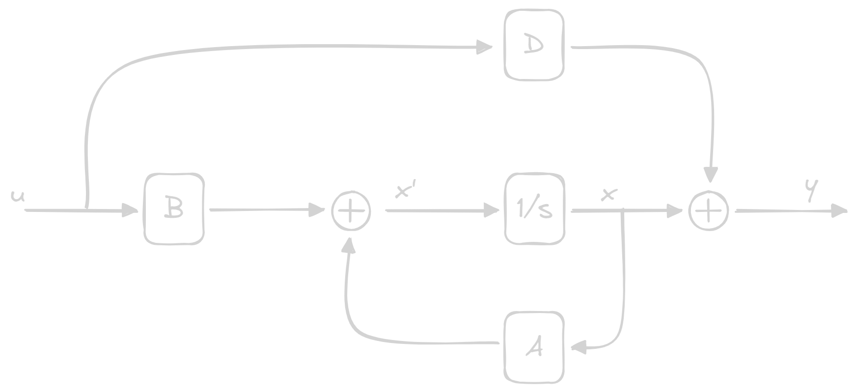
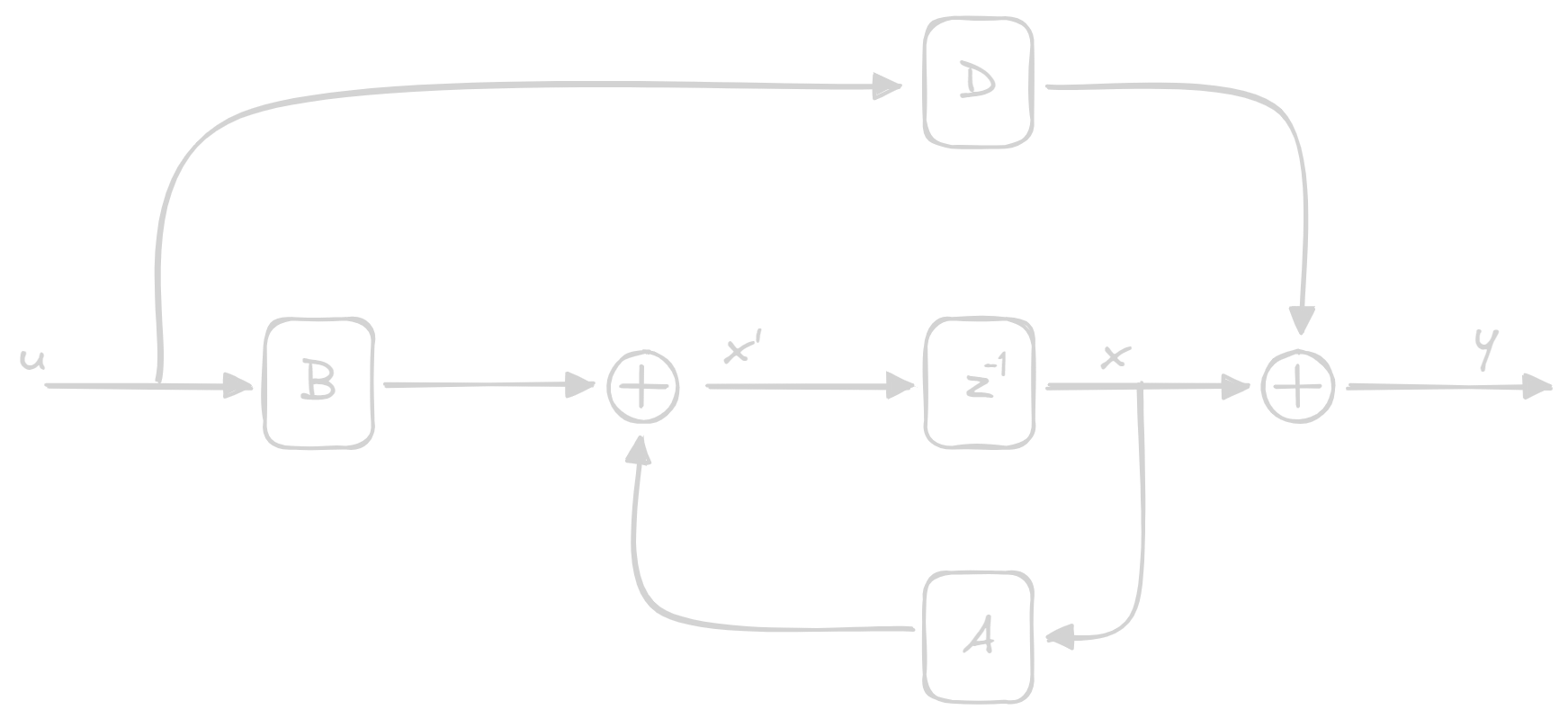
## State Space Representation

### State Matrices
A state space representation has 4 Matrices: $A, B, C, D$ with coefficients in 
$\R$:
- $A$: State Matrix `[x_rows, x_columns]`
- $B$: Input Matrix `[x_rows, u_columns]`
- $C$: Output Matrix `[y_rows, x_columns]`
- $D$: Direct Coupling Matrix `[y_rows, u_columns]`

$$
\begin{cases}
\dot{x}(t) = Ax(t) + Bu(t) \;\;\;\; \text{Dynamic of the system}\\
      y(t) = C{x}(t) + Du(t) \;\;\;\; \text{Static of the outputs}
\end{cases}
$$

This can be represented with the following diagrams:

#### Continuous Time:
![continuous state space diagram](../Images/Modern-Control/state-space-time.png)

---
#### Discrete time:

![discrete state space diagram](../Images/Modern-Control/state-space-discrete.png)

### State Vector
This is a state vector `[x_rows, 1]`:
$$
x(t) =  \begin{bmatrix}
            x_1(t)\\
            \dots\\
            x_x(t)
        \end{bmatrix}

\text{or} \:

x(k) =  \begin{bmatrix}
            x_1(k)\\
            \dots\\
            x_x(k)
        \end{bmatrix}
$$

Basically, from this we can know each next step of the state vector, represented 
as:

$$
x(k + 1) = f\left( 
    x(k), u(k)
\right) = Ax(k) + Bu(k)
$$

### Examples

#### Cart attached to a spring and a damper, pulled by a force
![cart being pulled image](../Images/Modern-Control/cart-pulled.png)

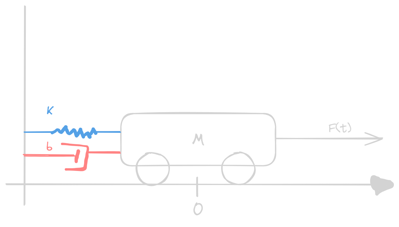
##### Formulas
- <span style="color:#55a1e6">Spring: $\vec{F} = -k\vec{x}$</span>
- <span style="color:#ff8382">Fluid Damper: $\vec{F_D} = -b \vec{\dot{x}}$</span>
- Initial Force: $\vec{F_p}(t) = \vec{F_p}(t)$
- Total Force: $m \vec{\ddot{x}}(t) =  \vec{F_p}(t) -b \vec{\dot{x}} -k\vec{x}$

> [!TIP]
>
> A rule of thumb is to have as many variables in our state as the max number
> of derivatives we encounter. In this case `2`
>
> Solve the equation for the highest derivative order
>
> Then, put all variables equal to the previous one derivated:
>
$$
x(t) =  \begin{bmatrix}
            x_1(t)\\
            x_2(t) = \dot{x_1}(t)\\
            \dots\\
            x_n(t) = \dot{x}_{n-1}(t)
        \end{bmatrix}
\;
\dot{x}(t) =  \begin{bmatrix}
            \dot{x_1}(t) = x_2(t)\\
            \dot{x_2}(t) = x_3(t)\\
            \dots\\
            \dot{x}_{n-1}(t) = \dot{x}_{n}(t)\\
            \dot{x}_{n}(t) = \text{our formula}
        \end{bmatrix}

$$


Now in our state we may express `position` and `speed`, while in our 
`next_state` we'll have `speed` and `acceleration`:
$$
x(t) =  \begin{bmatrix}
            x_1(t)\\
            x_2(t) = \dot{x_1}(t)
        \end{bmatrix}
\;
\dot{x}(t) =  \begin{bmatrix}
            \dot{x_1}(t) = x_2(t)\\
            \dot{x_2}(t) = \ddot{x_1}(t)
        \end{bmatrix}

$$
Our new state is then:
$$
\begin{cases}
\dot{x}_1(t) = x_2(t)\\
\dot{x}_2(t) = \frac{1}{m} \left( \vec{F}(t) - b x_2(t) - kx_1(t) \right)
\end{cases}
$$

let's say we only want to check for the `position` and `speed` of the system, our
State Space will be:
$$
A = \begin{bmatrix}
0 & 1 \\
- \frac{k}{m} & - \frac{b}{m} \\
\end{bmatrix}

B = \begin{bmatrix}
0 \\
\frac{1}{m} \\
\end{bmatrix}

C = \begin{bmatrix}
1 & 0 \\
0 & 1
\end{bmatrix}

D = \begin{bmatrix}
0
\end{bmatrix}
$$

let's say we only want to check for the `position` of the system, our
State Space will be:
$$
A = \begin{bmatrix}
0 & 1 \\
- \frac{k}{m} & - \frac{b}{m} \\
\end{bmatrix}

B = \begin{bmatrix}
0 \\
\frac{1}{m} \\
\end{bmatrix}

C = \begin{bmatrix}
1 & 0 
\end{bmatrix}

D = \begin{bmatrix}
0
\end{bmatrix}
$$

> [!TIP]
> In order to being able to plot the $\vec{x}$ against the time, you need to 
> multiply $\vec{\dot{x}}$ for the `time_step` and then add it to the state[^so-how-to-plot-ssr]
>

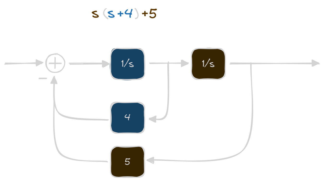
### Horner Factorization
let's say you have a complete polynomial of order `n`, you can factorize 
in this way:

$$
\begin{align*}
p(s) &= s^5 + 4s^4 + 5s^3 + 2s^2 + 10s + 1 =\\

&= s ( s^4 + 4s^3 + 5s^2 + 2s + 10) + 1 = \\

&= s ( s (s^3 + 4s^2 + 5s + 2) + 10) + 1 = \\

&= s ( s (s (s^2 + 4s + 5) + 2) + 10) + 1 = \\

&= s ( s (s ( s (s + 4) + 5) + 2) + 10) + 1

\end{align*}
$$

If you were to take each s with the corresponding number in the parenthesis, 
you'll make this block:
![horner factorization to diagram block](../Images/Modern-Control/horner-factorization.png)










### Case Studies
<!-- TODO: Complete case studies -->
- PAGERANK 
- Congestion Control
- Video Player Control
- Deep Learning
  
[^so-how-to-plot-ssr]: [Stack Exchange | How to plot state space variables against time on unit step input? | 05 January 2025 ](https://electronics.stackexchange.com/questions/307227/how-to-plot-state-space-variables-against-time-on-unit-step-input)