Control-Network-Systems/docs/Chapters/5-STATE-FEEDBACK.md

State Feedback

State Feedback

When you have your G(s), just put poles where you want them to be and compute the right k_i.

What we are doing is to put u(t) = -Kx(t), feeding back the state to the system.

Warning

While K matrix is controllable, the A matrix is equivalent to our plant, so it's impossible to change a_i without changing the system

Caution

We are doing some oversimplifications here, but this can't be used as formal proof for whatever we are saying. To see more, look at Ackerman's formula.

However is it possible to put a fictional reference input to make everything go back to a similar proof for the characteristic equation[^reference-input-pole-allocation]

While it is possible to allocate poles in each form, the Canonical Control one makes it very easy to accomplish this task:

A = \begin{bmatrix}
- a_1 \textcolor{#ff8382}{-k_1}& -a_2 \textcolor{#ff8382}{-k_2}
& -a_3 \textcolor{#ff8382}{-k_3}& \dots 
& -a_{n-1}\textcolor{#ff8382}{-k_{n-1}}
 &-a_n \textcolor{#ff8382}{-k_n}\\
1 & 0 & 0 & \dots  & 0 &  0\\
0 & 1 & 0 & \dots & 0 & 0\\
\dots & \dots & \dots & \dots  & \dots \\
0 & 0 & 0 & \dots & 1 & 0
\end{bmatrix}

This changes our initial considerations, however. The new Characteristi Equation becomes:

det\left(sI - (A - BK)\right)

State Observer

What happens if we have not enough sensors to get the state in realtime?

Note

Measuring the state involves a sensor, which most of the times is either inconvenient to place because of space, or inconvenient economically speaking

In this case we observe our output to estimate our state (\hat{x}). THis new state will be used in our G_c block:

\dot{\hat{x}} = A\hat{x} + Bu + L(\hat{y} - y) = A\hat{x} + Bu + 
LC(\hat{x} - x) 

Since we are estimating our state, we need the estimator to be fast, at least 6 times fater than our plant, and u = -K\hat{x}.

Let's compute the error we introduce in our system:

\begin{align*}
e &= x - \hat{x} \rightarrow \\
\rightarrow \dot{e} &= \dot{x} - \dot{\hat{x}}  \rightarrow\\

&\rightarrow Ax - BK\hat{x} - A\hat{x} + BK\hat{x} - LCe \rightarrow\\
&\rightarrow -Ae - LCe \rightarrow\\
&\rightarrow eig(-A-LC)
\end{align*} 

Making a Controller

So, this is how we will put all of these blocks saw until now.

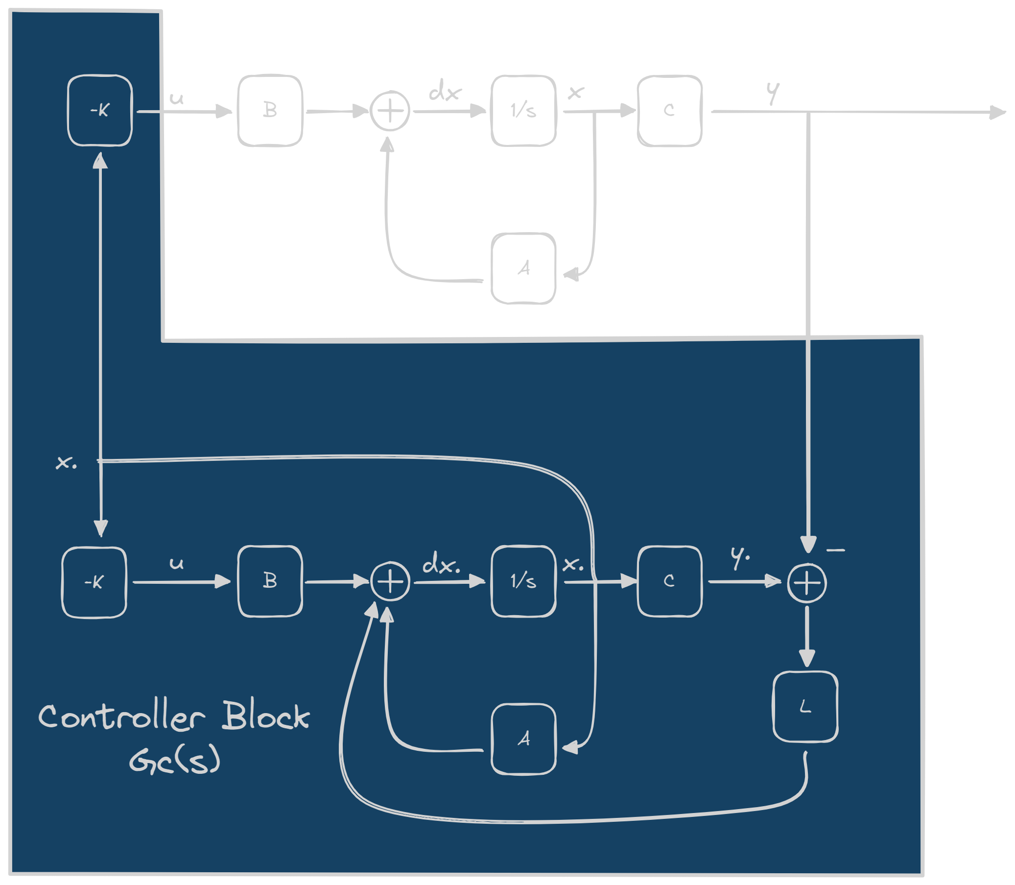
From this diagram we can deduce immediately that to us our input is y and our output is u. By treating the blue part as a black box, we can say that:

\begin{cases}
\dot{\hat{x}} = A\hat{x} - BK\hat{x} + LC\hat{x} - Ly \\
u = -K\hat{x}
\end{cases}

So our S(A_c, B_c, C_c, D_c) is:

\begin{align*}
&A_c = A_p - B_pK + LC_p \\
&B_c = -L \\
&C_c = -K \\
&D_c = 0 \\
\end{align*}

and so, you just need to substitute these matrices to the equation of the G_p(s) and you get you controller

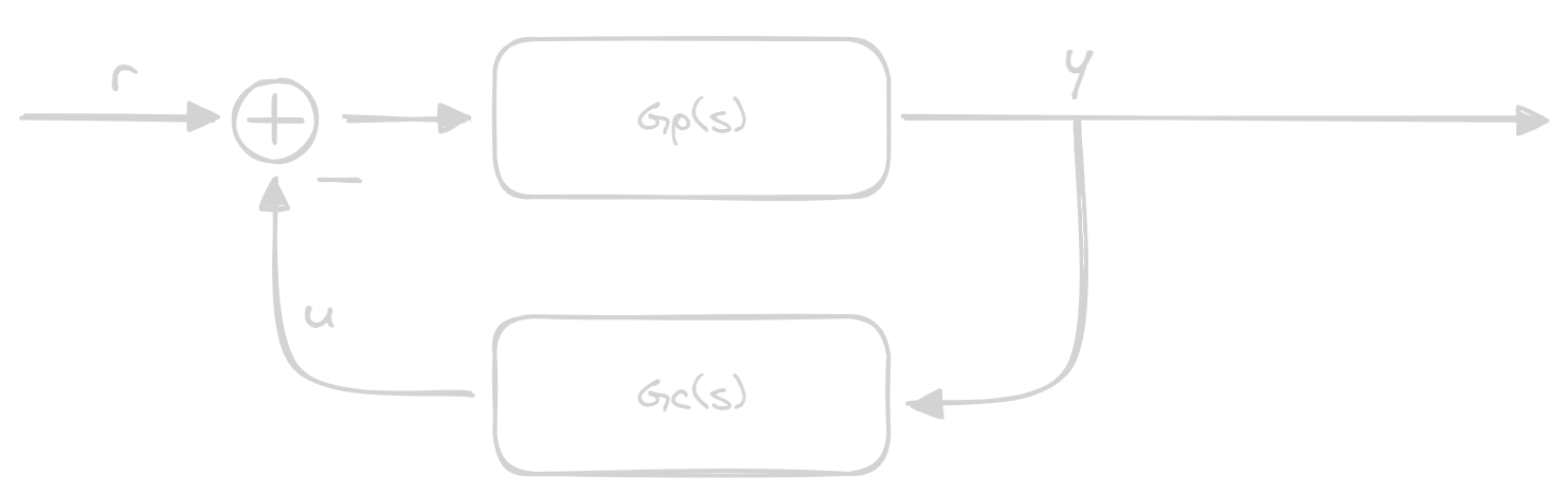
Inserting the reeference

Until now we've worked without taking the reference into consideration, so let's add it like we normally do:

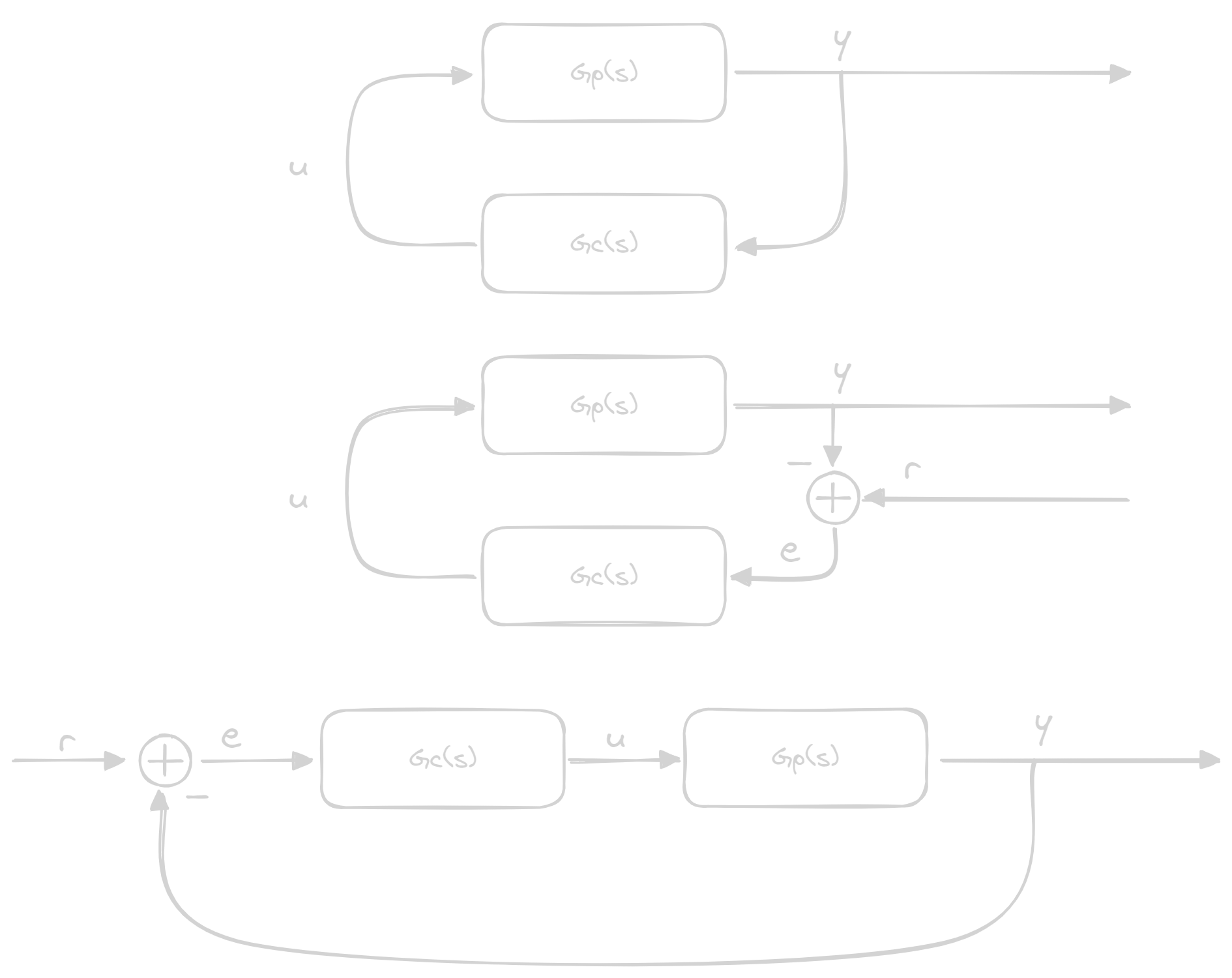
Here we can compute the error and our G(s) we have in our system:

e = r(t) - y(t) \\
G(s) = \frac{G_c(s)G_p(s)}{1 + G_c(s)G_p(s)}

Another way to deal with the reference is to put it between our blocks:

e = r(t) - \mathcal{L}^{-1}\left\{Y(s)G_c(s)\right\} \\
G(s) = \frac{G_p(s)}{1 + G_c(s)G_p(s)}

Now, let's see the difference in both G_1(s) and G_2(s):

\begin{align*}
G_1(s) &= \frac{G_c(s)G_p(s)}{1 + G_c(s)G_p(s)}  


\\


&= \frac{
    \frac{N_c}{D_c}\frac{N_p}{D_p}
}{
1 + \frac{N_c}{D_c} \frac{N_p}{D_p}
} \\


&= \frac{
    \frac{N_c N_p}{D_c D_p}
}{
    \frac{D_cD_p +N_cN_p}{D_cD_p} 
} \\


&= \frac{
    N_c N_p
}{
    D_cD_p +N_cN_p
} \\

\end{align*}
\;\;\;\;
\begin{align*}
G_2(s) &= \frac{G_p(s)}{1 + G_c(s)G_p(s)}  


\\


&= \frac{
    \frac{N_p}{D_p}
}{
1 + \frac{N_c}{D_c} \frac{N_p}{D_p}
} \\


&= \frac{
    \frac{N_p}{D_p}
}{
    \frac{D_cD_p +N_cN_p}{D_cD_p} 
} \\


&= \frac{
    N_c D_c
}{
    D_cD_p +N_cN_p
} \\

\end{align*}

While both have the same poles, they differ in their zeroes