Video Streaming

Nowadays video streaming works by downloading n chunks of a video v at different qualities l_{i}.

In order to model a device reproducing a video, we can consider the device having a buffer that has a dimension b_{max}. Whenever we play the video we are removing content from the buffer, making space for new chunks.

When the buffer is full, we don't donwload new chunks. When it's empty the reproduction will stop.

Our objective is to keep the buffer size in this range:


0 < b < b_{max}

Downard Spiraling

The reason why we should never get our buffer full is as we will stop using bandwidth. This means that if there's another greedy flow going on, it will perceive an increase in bandwidth, getting more and more of it.

This means that our video streaming will, on the contrary, perceive a lower bandwidth and the quality will drop.

Existing Protocols to Control Buffer Size

DASH (Dynamic Adaptive Streaming over Http)

HLS (Http Live Streaming)

Made by Apple, have a length of chunks equal to 10s

Controlling Video Streaming

First of all, we must say that Video Streaming should be controlled with a controller built-on-top of the TCP controller, as the TCP controller itself was built-on-top the IP controller, etc...

This is a generic scheme:

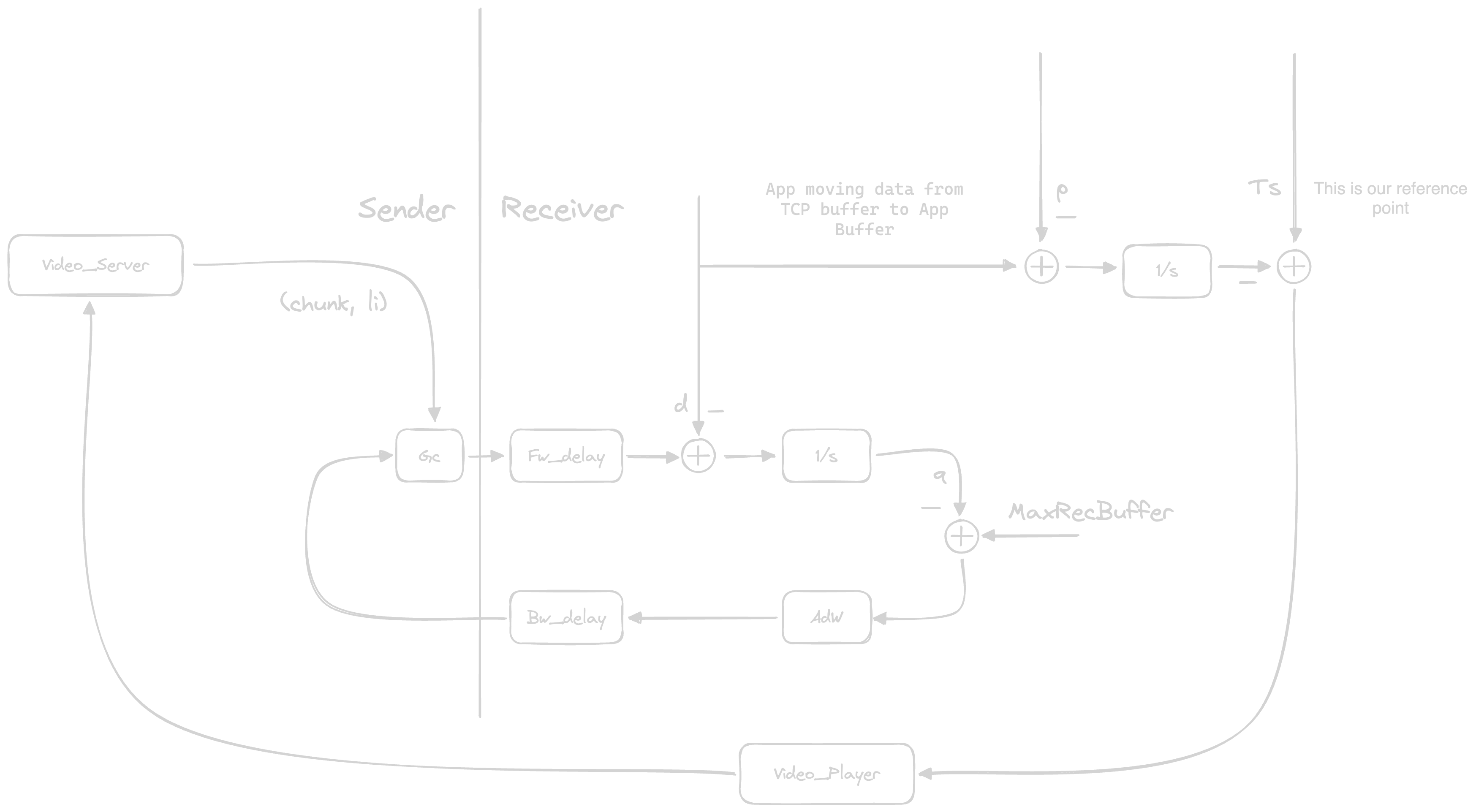
Our Player buffer must be measured in seconds!!!


\begin{align*}
r(t) &= \frac{
    \Delta D
}{
    \Delta t
} = \frac {
    \text{data\_quality}
}{
   \text{time\_interval}
} bps\\

\Delta t_f &= \text{frame\_time} \\
l(t) &= \frac{
    \Delta D
}{
    \Delta t_f
}bps = \text{coded\_movie} \\
t &= \text{real\_time} \\
t_f &= \text{move\_time} \\
\frac{
    \Delta t_f
} {
    \Delta t
} &= \left\{ 1, < 1, > 1\right\} \rightarrow 
\text{When we 1.5x or 0.5x on video} \\
\dot{t}_f &= \frac{dt_f}{dt}


\end{align*}

From here we have:


\begin{align*}
r(t) &= \frac{
    \Delta D
}{
    \Delta t
} = \frac{
    \Delta D
}{
    \Delta t
} 
\frac{
    \Delta t_f
}{
    \Delta t_f
} \\


&= \frac{
    \Delta D
}{
    \Delta t_f
} 
\frac{
    \Delta t_f
}{
    \Delta t
} \\


&= l(t)\dot{t}_f \\
\dot{t}_f &= \frac{r(t)}{l(t)}
\end{align*}

Now, let's suppose we are reproducing the video:


\dot{t}_f = \frac{r(t)}{l(t)} -o(t) \rightarrow \text{$o(t) = 1$ 1s to see 1s}

Tip

o(t) is just how many seconds we are watching per seconds. It basically depends on the multiplier of speed we put on the video:
0.5x -> 0.5s of video seen per second
2x   -> 2s of video seen per second
...

Feedback Linearization

Whenever we have a non-linear-system we can substitute the input for a function dependent on the state


\begin{align*}
\dot{x} &= f(x,u) \\
\dot{x} &= Ax + Bu(x)
\end{align*}

Coming back to our goal of controlling video streaming. We want to have a set point for our system t^s_f. As usual, we get the error and, in this case, we want to have a 0 position error over the input, so we add an integrator:


t_I = \int^t_{- \infty} t^s_f - t_f(\tau) d\tau

Because we have integrated, we are augmenting our state space


\begin{align*}
x &= \begin{bmatrix}
t_f = \frac{r(t)}{l(t)} - o(t)\\ 
t_I
\end{bmatrix} && \text{as we can see, $t_f$ is non linear} \\
\end{align*}

Because t_f is non linear, we must find a way to linearize it¹:


\frac{r(t)}{l(t)} - o(t) = k_pt_f + k_It_I \rightarrow \\
l(t) = \frac{
    r(t)
}{
    o(t) + k_pt_f + k_It_I
}

Now, simply, this algorithm will take the video quality that is nearer l(t)

3.8 KiB Raw Permalink Blame History