Deep-Learning/Chapters/11-GANs/INDEX.md

GANs

Pseudorandom Numbers

There are several alagorithms to generate random numbers on computers. These techniques are to have randomness over inputs to make experiments, but are still deterministic algorithms.

In fact, they take a seed that in turn generates the whole sequence. Now, if this seed is either truly random or not is not the goal. However the important thing is that for each seed there exists only one sequence of random values for an algorithm.

random_{seed = 12}(k) = random_{seed = 12}(k)

Caution

Never use these generators for crypthographical related tasks. There are ways to leak both the seed and the whole sequence, making any encryption or signature useless.

Cryptographically secure algorithms need a source of entropy, input that is truly random, that is external to the system (since computers are deterministic)

Pseudorandom Algorithms

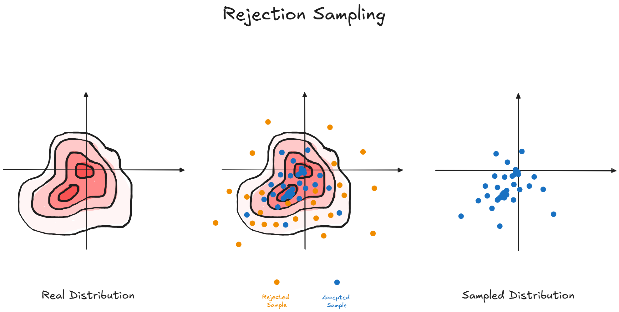
Rejection Sampling (aka Acceptance-Rejection Method)

Instead of sampling directly over the complex distribution, we sample over a simpler one, usually a uniform distribution, and accept or reject values according to some conditions.

If these conditions are crafted in a specific way, our samples will resemble those of the complex distribution

However we need to know the real probability distribution before being able to accept and reject samples.

Metropolis-Hasting

The idea is of constructing a stationary Markov Chain along the possible values we can sample.

Then we take a long journey and see where we end up. then we sample that point

Inverse Transform (aka Smirnov Transform)

The idea is of sampling directly from a well known distribution and then return a number from the complex distribution such that its probability function is higher than our simple sample

u \in \mathcal{U}[0, 1] \\
\text{take } x \text{ so that }  F(x) \geq u \text{ where } \\
F(x) \text{ is the the desired cumulative distribution function }

As proof we have that

F_{X}(x) \in [0, 1] = X \rightarrow F_{X}^{-1}(X) = x \in \R \\
\text{Let's define } Y = F_{X}^{-1}(U) \\
F_{Y}(y) =
    P(Y \leq y) =
    P(F_{X}^{-1}(U) \leq y) = P(F_{X}(F_{X}^{-1}(U)) \leq F_{X}(y)) =
    P(U \leq F_{X}(y)) = F_{X}(y)

In particular, we demonstrated that X and Y have the same distribution, so they are the same random variable. We also demonstrated that it is possible to define a random variable of a desired distribution, starting from another.

Tip

Another way to view this is by thinking of the uniform sample as the probability that we want from our target distribution.

When we find the smallest number that gives the same probability, it's like sampling from the real distribution (especially because we discretize).

By Davidjessop - Own work, CC BY-SA 4.0, Link

Note

The last passage says that a uniform variable is less than a value, that comes from a distribution. Since F_{U}(x) = P(U \leq x) = x the last part holds.

We can use the CDF of X in the probability function, without inverting the inequality because any CDF is positively monotone

Generative Models

Let's suppose for now that all similar things are ruled by a hidden probability distribution. This means that similar things live close together, but we don't know the actual distribution.

Let's say that we need to generate flower photos. To do so, we would collect several pictures of them. This allows us to infer a probability distribution that, while being different from the real one, it is still useful for our goal.

Now, to generate flower photos, we only need to sample from this distribution. However if none of the above methods are feasible (which is usually the case), we need to train a network capable of learning this distribution.

Direct Learning

This method consisits in comparing the generated distribution with the real one, e.g. see the MMD distance between them. However this is usually cumbersome.

Indirect Learning

We introduce the concept of a discriminator which will guess whether our image was generated or it comes from the actual distribution.

We then update our model based on the grade achieved by the discriminator

Generative Adversarial Networks

If we use the indirect learning approach, we need a Network capable of classificating generated and genuine content according to their labels.

However, for the same reasons of generative models, we don't have such a Network readily available, but rather we have to learn it.

The idea is that the discriminator learns to classify images (meaning that it will learn the goal distribution) and the generator learns to fool the discriminator (meaning that it will learn to generate according to the goal distribution)

Training Phases

We can train both the generator an discriminator together. They will backpropagate based on classification errors of the discriminator, however they will have 2 distinct objective:

• Generator: Maximize this error
• Discriminator: Minimize this error

From a game theory view, they are playing a zero-sum game and the perfect outcome is when the discriminator matches tags 50% of times

Loss functions

Assuming that G(\vec{z}) is the result of the generator, D(\vec{a}) is the result of the discriminator, y = 0 is the generated content and y = 1 is the real one

• Loss Function:
  This is the actual loss for the Discriminator, however we use the ones below to explain the antagonist goal of both networks. Here \vec{x} may be both.

\min_{D} \{
    \underbrace{
        -y \log{(D(\vec{x}))}
    }_{\text{Loss over Real Data}}
    \underbrace{
        - (1 -y)\log{(1-D(\vec{x}))}
    }_{\text{Loss over Generated Data}}
\}

Note

Notice that our generator can only control the loss over generated data. This will be its objective.

• Generator:
  We want to maximize the error of the Discriminator D(\vec{a}) when y = 0

\max_{G}\{ -(1 -y) \log(1 - D(G(\vec{z})))\} =
    \max_{G}\{- \log(1 - D(G(\vec{z})))\}

• Discriminator:
  We want to minimize its error when y = 1. However, if the Generator is good at its job D(G(\vec{z})) \approx 1 the equation above will be near 0, so we use these instead:

\begin{aligned}
\min_{G}\{ (1 -y) \log(1 - D(G(\vec{z})))\} &=
    \min_{G}\{\log(1 - D(G(\vec{z})))\} \\
    &\approx \max_{G}\{- \log(D(G(\vec{z})))\}
\end{aligned}

However they are basically playing a minimax game:

\min_{D} \max_{G} \{
- E_{x \sim Data} \log(D(\vec{x})) - E_{z \sim Noise} \log(1 - D(G(\vec{z})))
\}

In this case we want both scores balanced, so a value near 0.5 is our goal, meaning that both are performing at their best.

Note

Performing at their best means that the Discriminator is always able to classify correctly real data and the Generator is always able to fool the Discriminator.