Deep-Learning/Chapters/16-Energy-Based-Models/INDEX.md

Energy Based Models

These models takes 2 inputs, one of which is the . Then they are passed through another function that output their compatibility, or "goodness"¹. The lower the value, the better the compatibility.

The objective of this model is finding the most compatible value for the energy function across all possible values:

\hat{y} = \argmin_{y \in \mathcal{Y}}(E(x, \mathcal{Y})) \\
x \coloneqq \text{ network output | } \mathcal{Y} \coloneqq
\text{ set of possible labels}

The difficult part here is choosing said \hat{y} as the space \mathcal{Y} may be too large, or even infinite, and there could be multiple y that may have the same energy, so multiple solutions.

Since we want to model our function E(x, y), it needs to change according to some weights W. Since each time we change W we are changing also the output of E(x, y), we are technically defining a family of energy functions.

However, not all of them give us what we need, thus, by tuning W, we explore this space to find a E_W(x, y) that gives acceptable results.

During inference, since we will have built a function with a structure specifically crafted to be like that, we will generate a y^*_0 randomically and then we will update it through the gradient descent

Tip

If this thing is unclear, think that you have fixed your function E_{W} and notice that x is unchangeable too. During gradient descent, you can update the value of y^* by the same algorithm used for W.

Now, you are trying to find a minimum for E_W, meaning that y^* will be the optimal solution when the energy becomes 0 or around it.

Designing a good Loss¹

Note

• y_i: correct label for x_i
• y^*_i: lowest energy label
• \bar{y}_i: lowest energy incorrect label

Using the energy function

Since we want the energy for y_i to be 0 for x_i, everything else is a loss for us:

L_i(y_i, E_{W}(x_i, y_i)) = E_{W}(x_i, y_i)

However, this function does not increase energy for other example, possibly resulting in the constant function:

E_W(x_i, y_j) = 0 \,\, \forall i \in {X}, \forall j \in {Y}

In other words, it gives 0 for all possible labels, resulting in a collapsed plane where all energies are equal.

Generalized Perceptron Loss

Another way is to give a lower bound for point y_i and pushing away everything else:

L_i(y_i, E_{W}(x_i, y_i)) = E_{W}(x_i, y_i) - \min_{y \in \mathcal{Y}}E_{W}(x_i, y)

When the loss becomes 0, it means that both terms are equal, meaning that E(x_i, y_i) has the lowest value. However this doesn't imply that there's not anothe y_j so that E(x_i, y_i) = E(x_i, y_j), implying that this method is still susceptible to flat planes.

Good losses

To avoid the problem of a collapsed plane, we can use several losses:

• Hinge Loss
• Log Loss
• MCE Loss
• Square-Square Loss
• Square-Exponential Loss
• Negative Log-Likelihood Loss
• Minimum Empirical Error Loss

All of these operates to increase the distance between y_i and \bar{y}_i so that the "best incorrect answer" is at least margin away from the correct one(s).

Warning

Negative Log Likelihood makes the plane way too harsh, making it like a ravine where good values are in the ravine and bad ones are on top²

Energy Based Model Architectures

Caution

Here x, y may be scalars or vectors

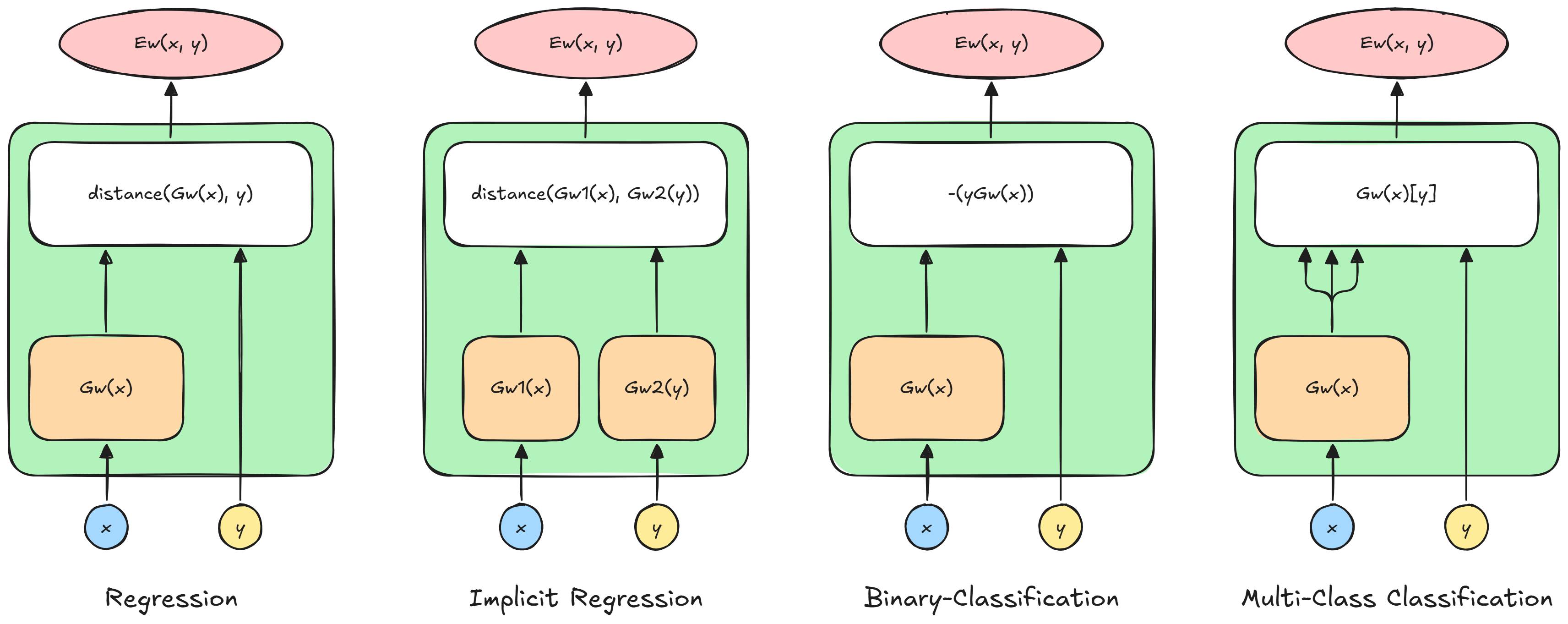
Regression

The energy function for a regression is simply:

E_W(x, y) = \frac{1}{2}|| G_W(x) - y ||_2^2

This architecture, during training will modify W so that G_W(x_i) \sim y_i and way different from all the other y_j. During inference, y^*_i will be the one that is the most similar to G_W(x_i)

Implicit Regression

We usually use this architecture when we want more than one possible answer. The trick is to map each admissible y to the same trasnformation of x_i:

E_W(x, y) = \frac{1}{2}|| G_{W_X}(x) -  G_{W_Y}(y) ||_2^2

During training both G_{W_X}(x_i) \sim G_{W_Y}(\mathcal{Y}_i), while during inference we will choose a value from \mathcal{Y}^*_i that will have the least energy

Binary Classification

For binary classification problems, we have:

E_W(x, y) = - yG_W(x)

During training it will make G_W(x_i) \gt 0 for y_i = 1 and viceversa. During inference, y_i^* will have the same sign of G_W(x_i).

Multi-Class Classification

For multiclass classification we will have:

E_W = \sum_{k = 0}^{C} \delta(y - k) \cdot G_W(x_i)_{[k]} \\
\delta(u) \coloneqq \text{ Kronecker impulse - } \begin{cases}
    1 \rightarrow u = 0 \\
    0 \rightarrow u \neq 0
\end{cases}

This is just a way to say that G_W(x_i) will produce several scores, an array of values, and the energy will be equal to the one for the class y_i.

During training G_W(x_i)_{[k]} \sim 0 for y_i = k and all the other will become high. During inference y^*_i = k for the lowest k^{th} value of G_W(x_i)

Latent-Variable Architectures

We introduce in the system a "latent" variable z that will help our model to get more details. We never receive this value, nor it is generated based on inputs³:

\hat{y}, \hat{z} = \argmin_{y,z} E(x, y, z)

However, if you like to find it only by looking at y and using a probabilistic approach, we get:

\hat{y} = \argmin_y \lim_{\beta \rightarrow \infin} - \frac{1}{\beta}
 \log \int_{z} e^{-\beta E(x, y, z)}

An advantage is that if we operate over a set \mathcal{Z}, we get a set \hat{\mathcal{Y}} of predictions. However, we need to limit the informativeness of our variable z, otherwise it is possible to perfectly predict y,

Relation between probabilities and Energy

We can think of energy and probablity of being the same thing, but over 2 different points of view:

P(y^* | x) = \frac{
    \underbrace{e^{-\beta E(x, y^*)}}_{\text{make energy small}}
}{
    \int_{y \in \mathcal{Y}} \underbrace{e^{-\beta E(x, y)}}_{
        \text{make energy big}}
}
\\
L(Y^*, W) = \underbrace{E_W(Y^*,X)}_{\text{make small}} + \frac{1}{\beta}
 \log \int_{y} \underbrace{e^{-\beta E(x, y)}}_{\text{make energy big}}

Note

• \text{gibbs distribution} \rightarrow e^{-\beta E(x, y^*)}
• \beta: akin to an inverse temperature

If you can avoid it, never work with probabilities, as they are often intractable and give less customization over the scoring function.

Warning

There may be reasons on why you would prefer having actual probabilities, rather than scores, and that's when you need 2 agents that need to interact with each other.

Since scores are calibrated only over the model we are working with, values across agents will differ, thus meaning different things.

However, this problem does not exist if the agents are trained end-to-end.

Contrastive-Methods

These methods have the objective of increasing energy for negative examples and lower it for positive examples

Basically we measure the distance, usually with a cosine similarity, and that becomes our energy function. Then we take a loss function that maximizes over similarity.

To make this method work, we need to feed it negative examples as well, otherwise we would not widen the dissimilarity between positive and negative examples.⁴

Note

There are also non contrastive methods that only uses positive examples, eliminating the need to get negative examples

Self Supervised Learning

It's a method of learning parts of data by other data parts. One example is BERT, or T5 that operates over Masked Language Tasks that involves predicting pieces of missing text, by looking at the remaining data.

---

1. A Tutorial on Energy-Based Learning ↩︎

2. Vito Walter Anelli | Ch. 15 pg. 17 | 2025-205 ↩︎

3. Youtube | Week 7 – Lecture: Energy based models and self-supervised learning | 22nd November 2025 ↩︎

4. DEEP LEARNING | Week 8 Ch. 8.1 | 22nd Novemeber 2025 ↩︎