Deep-Learning/Chapters/17-Flow-Generative-Models/INDEX.md

Flow Models

In generative modelling, what we are trying to achive is a remap of a known distribution, like a Guassian, to another distribution, like colors of pixels in face images.

le't imagine now that all distributions live in the same space, a bit like cities. Our objective is to make our citizen move from a city to another, thus we need to find the right mapping.

Vector field of a flow

Caution

Here we talk about speed, position and velocity. This is just an analogy to make the learning process smoother.

Let's sary that we have a flow, which in this context can be seen as the position function of \vec{x} at time t. The associated vector field is simply:

v_{t}(\vec{x}) = \frac{d \,\varphi_t(\vec{x})}{d \, t}\bigg \rvert_{t= 0}

This means that our vector field, read here as velocity, is the derivative of the flow, read as position, over time and evaluated at time t = 0. This means that we just need to know x_0, as the position at t = 0 is the initial position.

In particular, for the flow properties, we have that:

\begin{aligned}
    \varphi_t{(\vec{x})} &= \vec{x}(t) \\
    \varphi_0{(\vec{x})} &= \vec{x}_o \\
    \frac{d \,\varphi_t(\vec{x}_0)}{d \, t} &= f(\varphi_t(\vec{x}_0))
\end{aligned}

The last holds as the vector field is in function of t, thus even \vec{x} changes in function of time, and is equal to the flow.

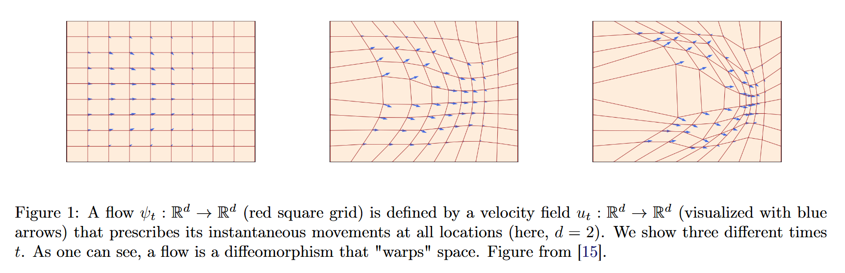
Image taken from An Introduction to Flow Matching and Diffusion Models

Note

As it is more evident by the image, the flow is basically a map of position of points. Since the position of each point changes over time, a flow warps space.

An interesting thing is that it gives us a snapshot of points are at time t.

Instead, the vector field v gives us how these position will be modified in the next pictures, giving us the instant velocity of all points, allowing us to predict where points will move before taking the next snapshot.

Mapping distributions via flow

It follows that a velocity function v can take x to a probability p only if it's flow goes there:

v_t \text{ generates } p_t \iff \mathcal{X}_t = \varphi_t(\mathcal{X}_0) \sim p_t

in other words, taken a random variable \mathcal{X_0}, we can say that is sampled from p_t at time t only if it goes into its probability boundaries.

Normalizing Flows

It is a technique in which we try to find several simple flows that will create a map of a distribution q to a distribution p.

Let's say that we want to learn a map T_W : q \rightarrow p, that we will call T_W\#q pushforward of q by T, we would need to minimize a Kullback-Leibler divergence:

\begin{aligned}
    D_{KL}(T_W\#q || p) &= \int_x \frac{\log(p(x))}{\log(T_W\#q(x))} p(x) dx = \\
        &= \underbrace{\int_x \log(p(x))p(x)\,dx}_\text{static, not controllable} -
        \underbrace{\int_x \log(T_W\#q(x))p(x)\,dx}_\text{modifiable}
\end{aligned}

Since we can ignore the static part, conditioned by only the true distribution, we take only the second part, which is equal to the expected value. We discretize it and we get

\mathbb{E_{x \sim p}}[\log(\,T_W\#q(x)\,)] = \sum_{x} \log(\,T_W\#q(x)\,)p(x)

Guess what, we have all these values, and this is similar to the Negative Log Likelihood, so, with a bit of notation changing, we get:

Loss(X, Y) = - \sum_{i}^{N} \log(T_W(\vec{x})^{(i)})

The thing is that we can't compute this directly, as there's no ground truth we can use to guide this. So, let's rewrite this in terms by applying the change of variables we get that:

p(\vec{y}) = q(T_W^{-1}(\vec{y})) \cdot \bigg | J_{T_W^{-1}}(\vec{y})\bigg |

Since it's complicated to derive T_W because it must be invertible and differential, this is simpler to achieve by composing T_W as T_W = \varphi_K \circ \dots \varphi_1. However these flows lose expressivity and they are complex to evaluate as K goes bigger.

Continuous Normalizing Flows

To solve the problem of expressivity, a solution is to solve the ODE with the euler method

Flow Matching

The idea is to train a velocity function that will bring us to the right distribution, and this is our flow matching. By treating it like an energy based model, we get:

E_t(\mathcal{X}_0, \mathcal{X}_1) =
    || v^W_t(\mathcal{X}_t) - v_t(\mathcal{X}_t) ||^2

Since we need our point to travel how we want it, we influence its velocity. Thus, by minimizing this error, we get the target trajectory.

However, there's a problem... We don't know v_t(\mathcal{X}_t) and we must find a method to derive it

Midpoint Method (aka Modified Euler's method)

The actual algorithm from wikipedia is:

y_{n + 1} = y_{n} + hf\left(y_n + \frac{h}{2}f(y_n, t_n), t_n + \frac{h}{2}\right)

translated to code becomes:

# Technically its velocity, not speed
#   velocity:   vector
#   speed:      magnitude
def compute_speed(old_position: list[], current_time: float) -> list[]:
    # this function is what
    #   we want to find
    pass

def compute_new_position(
    old_position: list[],
    old_speed: list[],
    current_time: float,
    time_step: float
):
    step = time_step / 2

    half_point_speed = compute_speed(
        old_position + step * old_speed,
        time + step
    )

    new_pos = old_position + step * half_point_speed
    return new_pos

Obviously we don't know what the speed function is, thus we just need to learn it. Now, inverting the formula we get that (with some abuse of notations) our target velocity in that point is:

f_{t + \frac{h}{2}} = \frac{y_{n + 1} - y_n}{h}

And since during training time we can compute this, as we have both y_n and y_{n+1}, we just need to set h to an arbitrary value, say 1 and we can easily compute this.

Now, we just need to learn the velocity function, and this is just the gradient descent of the difference between our learnt function and the computed one. Then, if we want to use an energy model, we get:

E_t(\mathcal{X}_0, \mathcal{X}_1) =
    || v^W_t(\mathcal{X}_t) - (\mathcal{X}_1 - \mathcal{X}_0) ||^2

Note

There's another method, applying Markov chains, though it's basically a flow matching with Euler's standard method where h \rightarrow \infty and so has multiple steps

Caution

This method is perfectly equivalent with using a conditional flow matching where z is sampled from a dirac distribution (basically a Normal distribution with \sigma = 0)

Conditional Flow Matching

Now, let's say that we want to describe the velocity v in other ways, the problem is that there isn't a unique path to go from q to p

GIF taken from https://dl.heeere.com/conditional-flow-matching/blog/conditional-flow-matching/

So the problem is now to describe this probability path over time. However we don't know p analytic function, but just a bunch of data points sampled from it.

The idea to solve this is to define a probability path, read velocity, that is conditioned by a variable z, conditioning variable, so that it is p(x | t, z), so that, once we choose a particular z, we get a p(x | t) that brings x from q to p and that has an analytic form.

The trick here is to find the probability p(x, t) by marginalizing over p(x |t, z). In practice this means that we just have to sum (or integrate) over all possible z values.

Since z is a random variable, a couple of techniques are one of sampling from a Linear Interpolation, or from a conical gaussian path¹

\text{Linear Interpolation} \\
\begin{cases}
    \mu = (1 - t)\cdot x_q + t \cdot x_p \\
    \sigma = 0 \\
    p(x | t, z = (x_q, x_p)) = \mathcal{N}(\mu, \sigma^2 I) \\
\end{cases}
\\
\text{ }
\\
\text{Velocity} \rightarrow v(x, t) = x_p - x_q
\\
\text{ }
\\
\text{ }
\\
\text{Conical Gaussian Path} \\
\begin{cases}
    \mu =  t \cdot x_p \\
    \sigma = (1 - t)^2 \\
    p(x | t, z = (x_p)) = \mathcal{N}(\mu, \sigma^2 I) \\
\end{cases}
\\
\text{ }
\\
\text{Velocity} \rightarrow v(x, t) = \frac{x - x_p}{1 - t}

To find the velocity, it's possible to use the continuity equation

Conditional Optimal Flow

One thing that could happen during the construction of our paths is that they cross. To solve this problem, we may choose couples of data such that they are coupled. This means that they won't cross.

In practice we only use minibatch Optimal Transport as it's costly to compute

ReFlow

Technically speaking a reflow is nothing more than what we already saw in flow matching². The difference lies in how we retrain the model and how we sample points.

We first train a model like in flow matching, and then we train another model where true labels are not provided. In fact the taget lables provided will come from our original model.

While we normally would think that our original model learnt corssing trajectories, this is not the case. Plus, a better sampling provided by chaning euler to 4th-order Runge-Kutta, we provide a better integration method.

By combining both techniques, our reflowed model will learn straighter trajectories.

Warning

It's not necessary that the 2 models are different or equal, nor you need to re-use the former model weights.

Guidance for generation

As for diffusion, we now know how to generate the target distribution, but what if the target distribution is the distribution of valid images and we want a picture of a dog?

Classifier Guidance

We could take our unconditioned model and use a classifier, plus another input used to guide, to change our model parameters (so, our velocity). However this means that we need a classifier that tells us if our generated output matches the label or not:

v_{W, t}(x | y) = v(x) + wb_t \nabla \log p_{Y |t}(y | x)

This means that our new velocity will be influenced by the weighted conditioned probability of obtaining y starting from x. Now we don't need to retrain our model from 0.

Since we are tuning 2 different models together, their magnitudes do not combine well, leading to potential problems. Moreover the classifier is not "perfect", so we need to consider its errors as well

Classifier Free Guidance

Instead of using a classifier, we can fine retrain our model to consider conditioning. Starting from the classifier equation for the velocity, we can demonstrate that:

u_{W, t}(x | y) = (1 - w)v(x) + w \cdot v(x | y)

Now, we can reuse the previous model and we will retrain it by passing y = \emptyset \text{ or } y \in \mathcal{Y} with probability \eta for being empty.

Once retrained, during inference can sample by using this formula, where y = \emptyset if it comes from an unguided sampling and y \in \mathcal{Y} if it's unguided.

d X_t = [(1 - w)v_{W, t}(X_t | \emptyset) + wv_{W, t}(X_t | y)] dt \\
w > 1

As you can notice, since w > 1, we are slowing the conditioned velocity with the unconditioned velocity, that is dampened. Moreover, if the prompt is unconditioned, this would be equal to the unmodified unconditional velocity.

Stable Diffusion 3

References

• An Introduction to Flow Matching and Diffusion Models
• Introduction to Flow Matching and Diffusion Models
• A Visual Dive into Conditional Flow Matching
• Rectified Flow
• An introduction to Flow Matching
• Flow With What You Know
• Diffusion Meets Flow Matching

---

1. A Visual Dive into Conditional Flow Matching | 26th November 2025 ↩︎

2. Flow With What You Know | 26th November 2025 ↩︎