Deep-Learning/Chapters/8-Recurrent-Networks/INDEX.md

Recurrent Networks | RNNs¹

Why would we want Recurrent Networks?

To deal with sequence related jobs of arbitrary length.

In fact they can deal with inputs of varying length while being fast and memory efficient.

While autoregressive models always needs to analyse all past inputs (or a window of most recent ones), at each computation, RNNs don't, making them a great tool when the situation permits it.

A bit of History²

In order to predict the future, we need information of the past. This is the idea behind RNNs for predicting the next item in a sequence.

While it has been attempted to accomplish this prediction through the use of memoryless models, they didn't hold up to expectations and had several limitations such as the dimension of the "past" window.

• Autoregressive Models
• Feed-Forward Neural Networks

Shortcomings of previous attempts²

• The context window was small, thus the model couldn't use distant past dependencies
• Some tried to count words, but it doesn't preserve meaning
• Some tried to make the context window bigger but this caused words to be considered differently based on their position, making it impossible to reuse weights for same words.

RNNs³

The idea behind RNNs is to add memory as a hidden-state. This helps the model to "remember" things for "long time", but since it is noisy, the best we can do is to infer its probability distribution, doable only for:

• Linear Dynamical Systems
• Hidden Markov Model

While these models are stochastic, technically the a posteriori probability ditstibution is deterministic.

Since we can think of RNNs hidden state equivalent to a a posteriori probability ditstibution, they are deterministic

Neurons with Memory⁴

While in normal NNs we have no memory, these neurons have a hidden-state, \vec{h} , which is fed back to the neuron itself.

The formula of this hidden-state is:

\vec{h}_t = f_{W}(\vec{x}_t, \vec{h}_{t-1})

In other words, The hidden-state is influenced by a function modified by weights and dependent by current inputs and preious step hidden-states.

For example, let's say we use a \tanh activation-function:

\vec{h}_t = \tanh(
    W_{h, h}^T \vec{h}_{t-1} + W_{x, h}^T \vec{x}_{t}
)

And the output becomes:

\vec{\bar{y}}_t = W_{h, y}^T \vec{h}_{t}

Note

Technically speaking, we could consider RNNs as deep NNs⁵

Different RNNs configurations

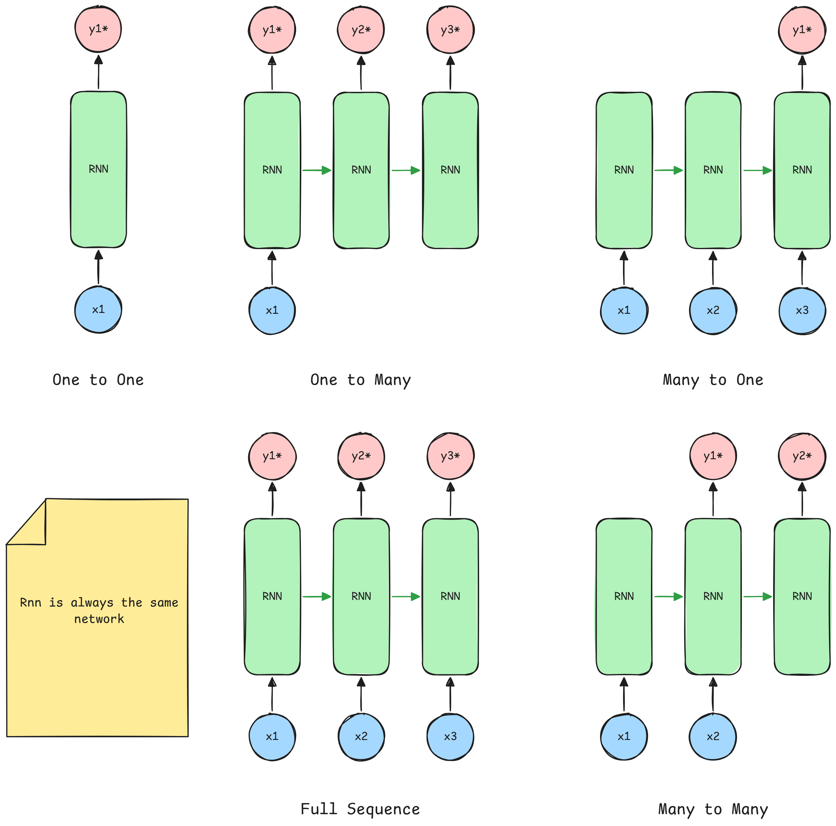
Providing initial-states for the hidden-states⁶

• Specify initial-states of all units
• Specify initial-states for a subset of units
• Specify initial-states for the same subset of units for each timestep (Which is the most naural way to model sequential data)

In other words, it depends on how you need to model data according to your sequence.

Teaching signals for RNNs⁷

• Specify desired final activity for all units
• Specify desired final activity for all units ofr the last few steps
  • This is good to learn attractors
  • Makes it easy to add extra error derivatives
• Speficfy the desired activity of a subset of units
  • The other units will be either inputs or hidden-states, as we fixed these

In other words, it depends on which kind of output you need to be produced.

for example, a sentimental analysis would need to have just one output, while a seq2seq job would require a full sequence.

Transforming Data for RNNs

Since RNNs need vectors, the ideal way to transform inputs into vectors is either having 1-hot encoding over whole words or transform them into tokens and then 1-hot encode them.

While this is may be enough, there's a better way where we transform each 1-hot encoded vector into a learned vector of fixed size (usually of smaller dimensions) during the embedding phase.

To better understand this, imagine a vocabulary of either 16K words or Tokens. we would have 16K dimensions for each vector, which is massive. Instead, by embedding it into 256 dimensions we can save both time and space complexity.

RNNs Training

Since RNNs can be considered a deep-layered NN, then we firstly train the model over the sequence and then backpropagate, keeping track of the training stack, adding derivatives along time-steps

Caution

If you have big gradients, remember to clip them

The thing is that is difficult to train RNNs on long-range dependencies because the gradient will either vanish or explode⁸

Mitigating training problems in RNNs

In order to mitigate these gradient problems that impairs our network ability to gain valuable information over long term dependencies, we have these solutions:

• LSTM:
  Make the model out of little modules crafted to keep values for long time
• Hessian Free Optimizers:
  Use optimizers that can see the gradient direction over smaller curvatures
• Echo State Networks⁹:
  The idea is to use a sparsely connected large untrained network to keep track of inputs for long time, while eventually be forgotten, and have a trained readout network that converts the echo output into something usable
• Good Initialization and Momentum:
  Same thing as before, but we learn all connections using momentum

Warning

long-range dependencies are more difficult to learn than short-range ones because of the gradient problem.

Gated Cells

These are neurons that can be controlled to make them learn or forget chosen pieces of information

Caution

With chosen we intend choosing from the hyperspace, so it's not really precise.

High Level Scheme

The point of an RNN cell is to be able to modify its internal state.

As for the image, this can be implemented by having gates (AND operations) to read, write and keep (remember) pieces of information in the memory.

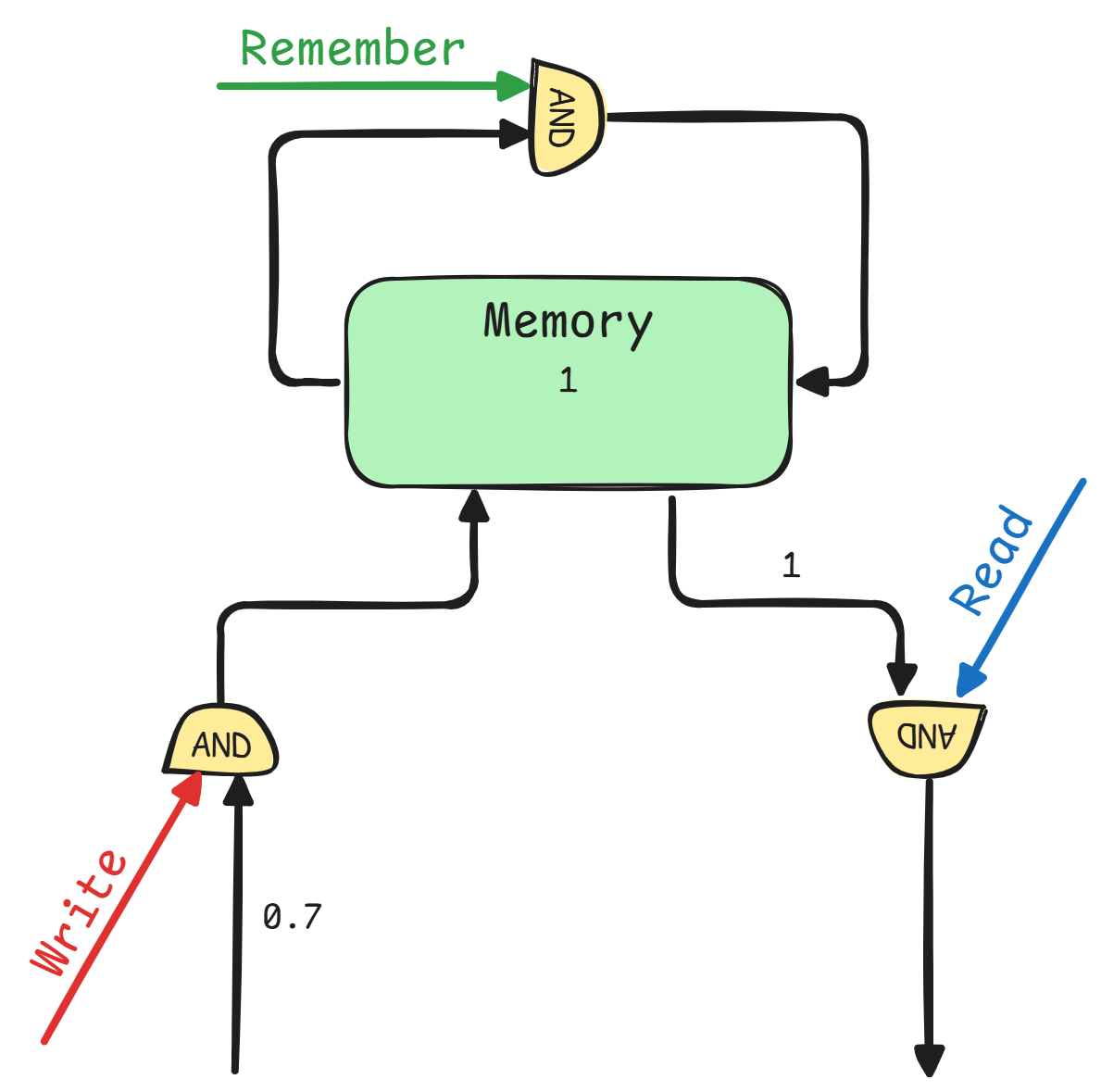
Even though this is a high level and simplistic architecture, it gives a rough idea of how to implement it.

• First of all, instead of using AND gates, we can substitute with an elementwise multiplication.

• Secondly we can implement an elementwise addition to take combine a new written element with a past one

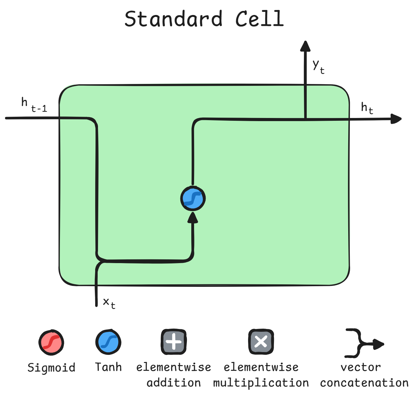
Standard RNN Cell

This is the most simple type of implementation. Here all signals are set to 1

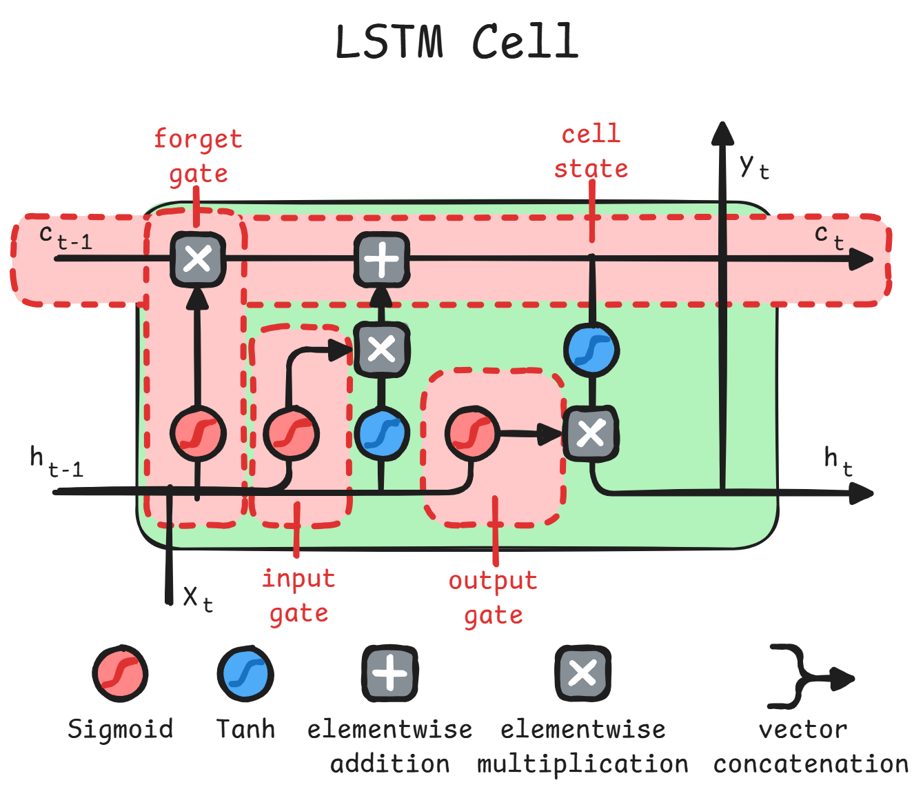
Long Short Term Memory | LSTM¹⁰¹¹

This cell has a separate signal, namely the cell-state, which controls gates of this cells, always initialized to 1.

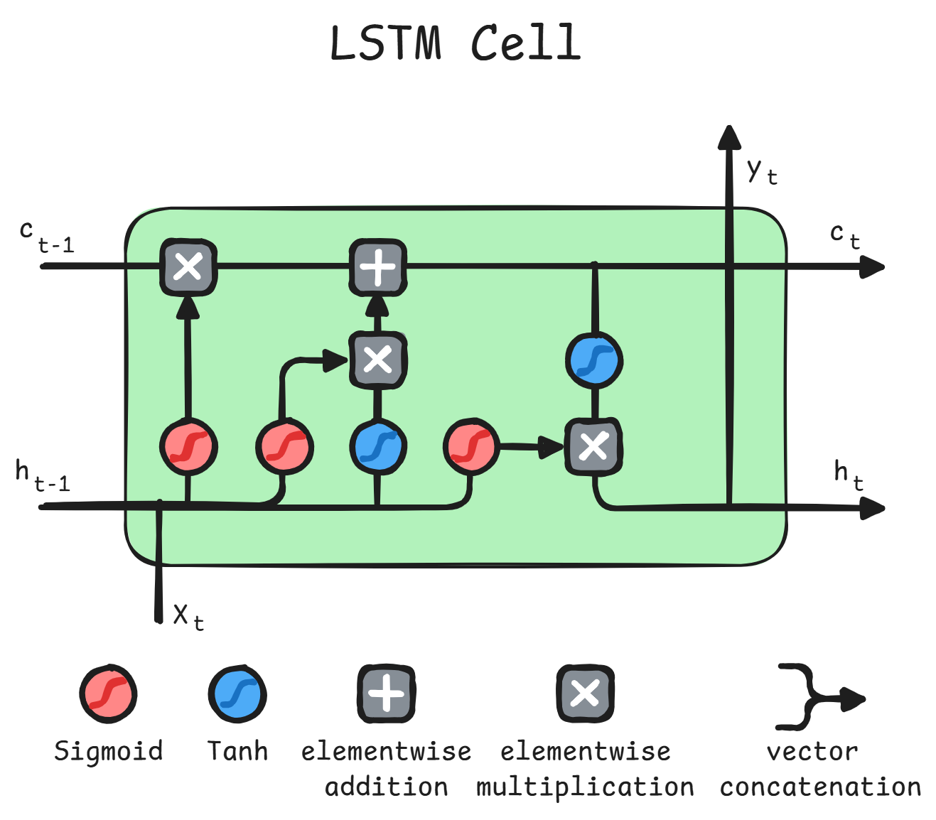
As for the image, we can identify a keep (or forget) gate, write gate and read gate.

• Forget Gate:
  The previous read state (h_{t-1}) concatenated with input (x_{t}) is what controls how much of the previous cell state keeps being remembered. Since it has values \in [0, 1], it has been called forget gate

• Input Gate:
  It is controlled by a sigmoid with the same inputs as the forget gate, but with different weights. It regulates how much of the tanh of same inputs goes into the cell state.

  tanh here has an advantage over the sigmoid for the value as it admits values \in [-1, 1]

• Output Gate:
  It is controlled by a sigmoid with the same inputs as the previous gates, but different weights. It regulates how much of the tanh of the current state cell goes over the output

Note

W will be weights associated with \vec{x} and U with \vec{h}.

The cell-state has the same dimension as the hidden-state

\odot is the Hadamard Product, also called the pointwise product

Forget Gate | Keep Gate

This gate controls the cell-state:

\hat{c}_{t} = \sigma \left(
    U_fh_{t-1} + W_fx_t + b_f
\right) \odot c_{t-1}

The closer the result of \sigma is to 0, the more the cell-state will forget that value, and opposite for values closer to 1.

Input Gate | Write Gate

controls how much of the input gets into the cell-state

c_{t} = \left(
    \sigma \left(
        U_ih_{t-1} + W_ix_t + b_i
    \right) \odot \tanh \left(
        U_ch_{t-1} + W_cx_t + b_c
    \right)
\right) + \hat{c}_{t}

The results of \tanh are new pieces of information. The higher the \sigma_i, the higher the importance given to that info.

Note

The forget gate and the input-gate are 2 phases of the update-phase.

Output Gate | Read Gate

Controls how much of the hidden-state is forwarded

h_{t} = \tanh (c_{t}) \odot \sigma \left(
    U_oh_{t-1} + W_ox_t + b_o
\right)

This produces the new hidden-state. Notice that the info comes from the cell-state, gated by the input and previous-hidden-state

---

Here the backpropagation of the gradient is way simpler for the cell-states as they require only elementwise multiplications

GRU¹²¹³

It is another type of gated-cell, but, on the contrary of LSTM-cells, it doesn't have a separate cell-state, but only the hidden-state, while keeping similar performances to LSTM.

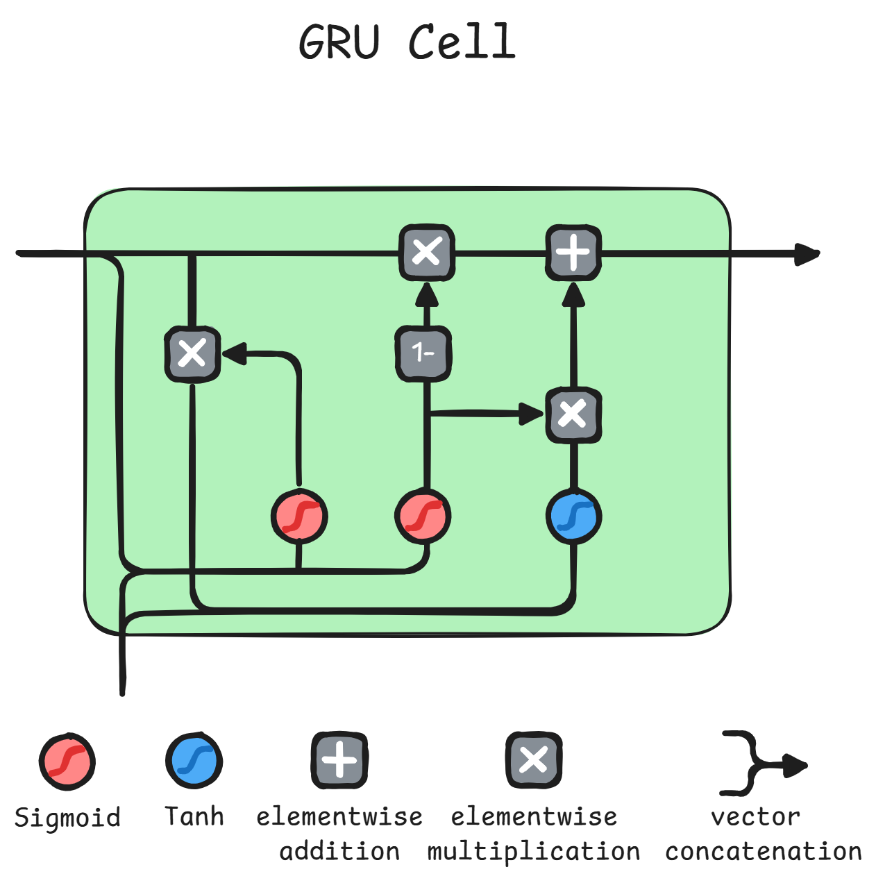
As for the image, we have only 2 gates:

• Reset Gate:
  Tells us how much of the old information should pass with the input. It is controlled by the old state and the input.
• Update Gate:
  Tells us how much of the old info will be kept and how much of the new info will be learnt. It is controlled by a concatenation of the output of reset gate and the input passing from a tanh.

Note

GRU doesn't have any output-gate and h_0 = 0

Update Gate

This gate unifies forget gate and input gate

\begin{aligned}

    \hat{h}_t &= \left(
        1 - \sigma \left(
            U_z h_{t-1} + W_z x_{t} + b_z
        \right)
    \, \right) \odot h_{t-1}
\end{aligned}

Reset Gate

This is what breaks the information flow from the previous hidden-state.

\begin{aligned}
    \bar{h}_t &= \sigma\left(
            U_r h_{t-1} + W_r x_{t} + b_r
        \right) \odot h_{t-1}
\end{aligned}

New hidden-state

\begin{aligned}
    h_t = \hat{h}_t + (\sigma \left(
        U_z h_{t-1} + W_z x_{t} + b_z
    \right) \odot \tanh \left(
        U_h \bar{h}_t + W_h x_t + b_h
    \right))
\end{aligned}

Tip

There's no clear winner between GRU and LSTM, so try them both, however the former is easier to compute

Bi-LSTM¹⁴¹⁵

We implement 2 networks, one that takes hidden states coming from computing info over in order, while the other one taking hidden states in reverse order.

Then we take outputs from both networks and compute attention and other operations, such as softmax and linear ones, to get the output.

In this way we gain info coming from both directions of a sequence.

Applications¹⁶

• Music Generation
• Sentiment Classification
• Machine Translation
• Attention Mechanisms

Pros, Cons and Quirks

References

• ai-master.gitbooks.io
• stanford.edu - CS224d-Lecture8
• deepimagesent
• introduction-to-rnns
• implementing-a-language-model-rnn-with-python-numpy-and-theano
• rnn-effectiveness
• Understanding-LSTMs

---

1. Vito Walter Anelli | Deep Learning Material 2024/2025 | PDF 8 ↩︎

2. Vito Walter Anelli | Deep Learning Material 2024/2025 | PDF 8 pg. 11 to 20 ↩︎

3. Vito Walter Anelli | Deep Learning Material 2024/2025 | PDF 8 pg. 21 to 22 ↩︎

4. Vito Walter Anelli | Deep Learning Material 2024/2025 | PDF 8 pg. 25 ↩︎

5. Vito Walter Anelli | Deep Learning Material 2024/2025 | PDF 8 pg. 43 to 47 ↩︎

6. Vito Walter Anelli | Deep Learning Material 2024/2025 | PDF 8 pg. 50 ↩︎

7. Vito Walter Anelli | Deep Learning Material 2024/2025 | PDF 8 pg. 51 ↩︎

8. Vito Walter Anelli | Deep Learning Material 2024/2025 | PDF 8 pg. 69 to 87 ↩︎

9. UniPI | ESN | 25th October 2025 ↩︎

10. Vito Walter Anelli | Deep Learning Material 2024/2025 | PDF 8 pg. 91 to 112 ↩︎

11. LSTM | Wikipedia | 27th April 2025 ↩︎

12. Vito Walter Anelli | Deep Learning Material 2024/2025 | PDF 8 pg. 113 to 118 ↩︎

13. GRU | Wikipedia | 27th April 2025 ↩︎

14. Vito Walter Anelli | Deep Learning Material 2024/2025 | PDF 8 pg. 127 to 136 ↩︎

15. Bi-LSTM | StackOverflow | 27th April 2025 ↩︎

16. Vito Walter Anelli | Deep Learning Material 2024/2025 | PDF 8 pg. 119 to 126 ↩︎