Deep-Learning/Chapters/10-Autoencoders/INDEX.md

Autoencoders

Here we are trying to make a model to learn an identity function without making it learn the actual identity function

h_{\theta} (x) \approx x

Now, if we were just to do this, it would be very simple, just pass the input directly to output.

The innovation comes from the fact that we can compress data by using an NN that has less neurons per layer than input dimension, or have less connections (sparse)

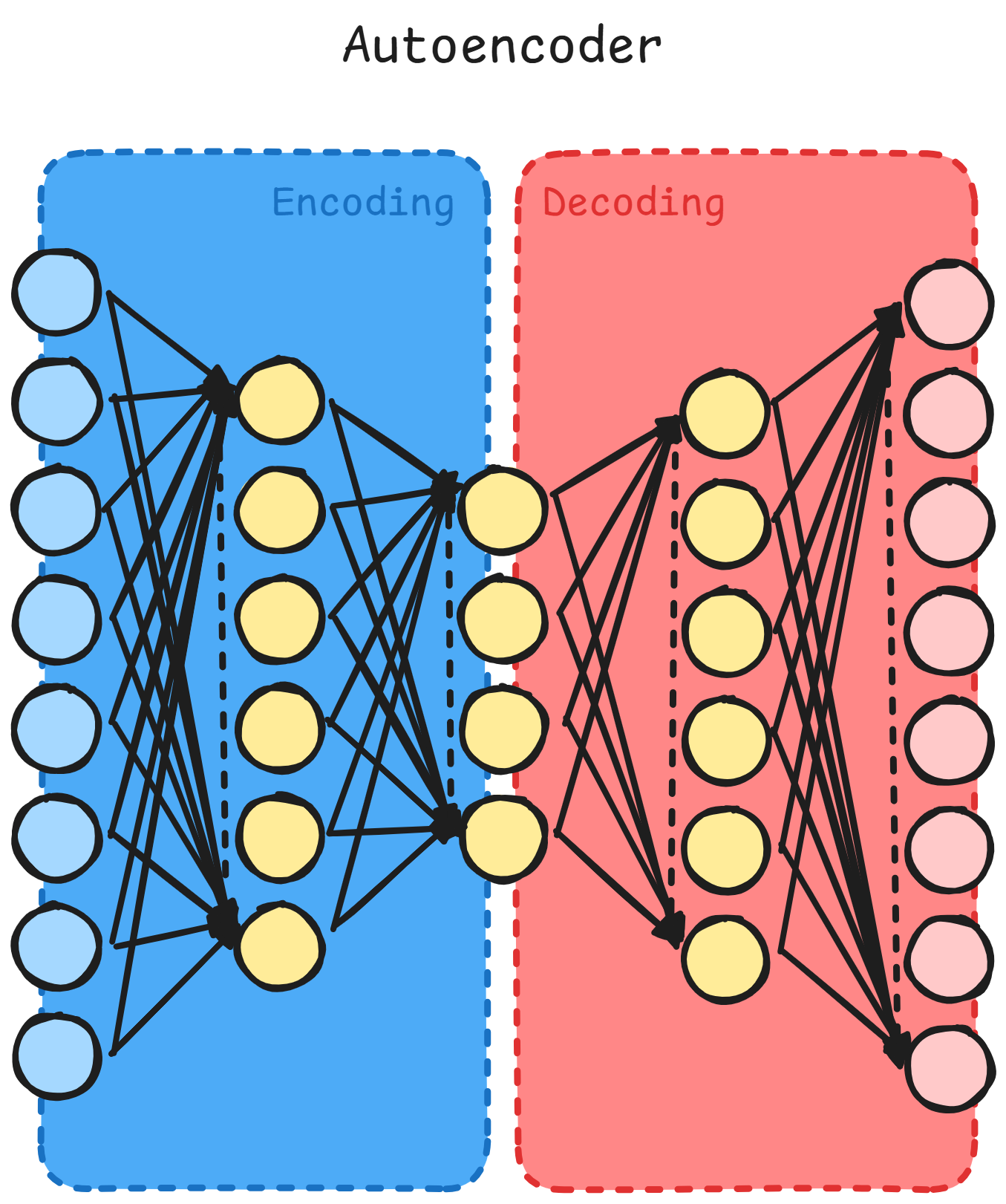
Compression

In a very simple fashion, we train a network to compress \vec{x} in a more dense vector \vec{y} and then later expand it into \vec{z}, also called prediction of \vec{x}

\begin{aligned}
    \vec{x} &= [a, b]^{d_x} \\
    \vec{y} &= g(\vec{W_{0}}\vec{x} + b_{0}) \rightarrow \vec{y} = [a_1, b_1]^{d_y} \\
    \vec{z} &= g(\vec{W_{1}}\vec{y} + b_{1}) \rightarrow \vec{z} = [a, b]^{d_x} \\
    \vec{z} &\approx \vec{x}
\end{aligned}

Sparse Training

A sparse hidden representation comes by penalizing values assigned to neurons (weights).

\min_{\theta}
\underbrace{||h_{\theta}(x) - x ||^{2}}_{\text{
    Reconstruction Error
}} +
\underbrace{\lambda \sum_{i}|a_i|}_{\text{
    L1 sparsity
}}

The reason on why we want sparsity is that we want the best representation in the latent space, thus we want to avoid our network to learn the identity mapping

Layerwise Training

To train an autoencoder we train layer by layer, minimizing the vanishing gradients problem.

The trick is to train one layer, then use it as the input for the other layer and training over it as if it were our x. Rinse and repeat for 3 layers approximately.

If you want, at last, you can put another layer that you train over data to fine tune

Tip

This method works because even though the gradient vanishes, since we already trained our upper layers, they already have working weights

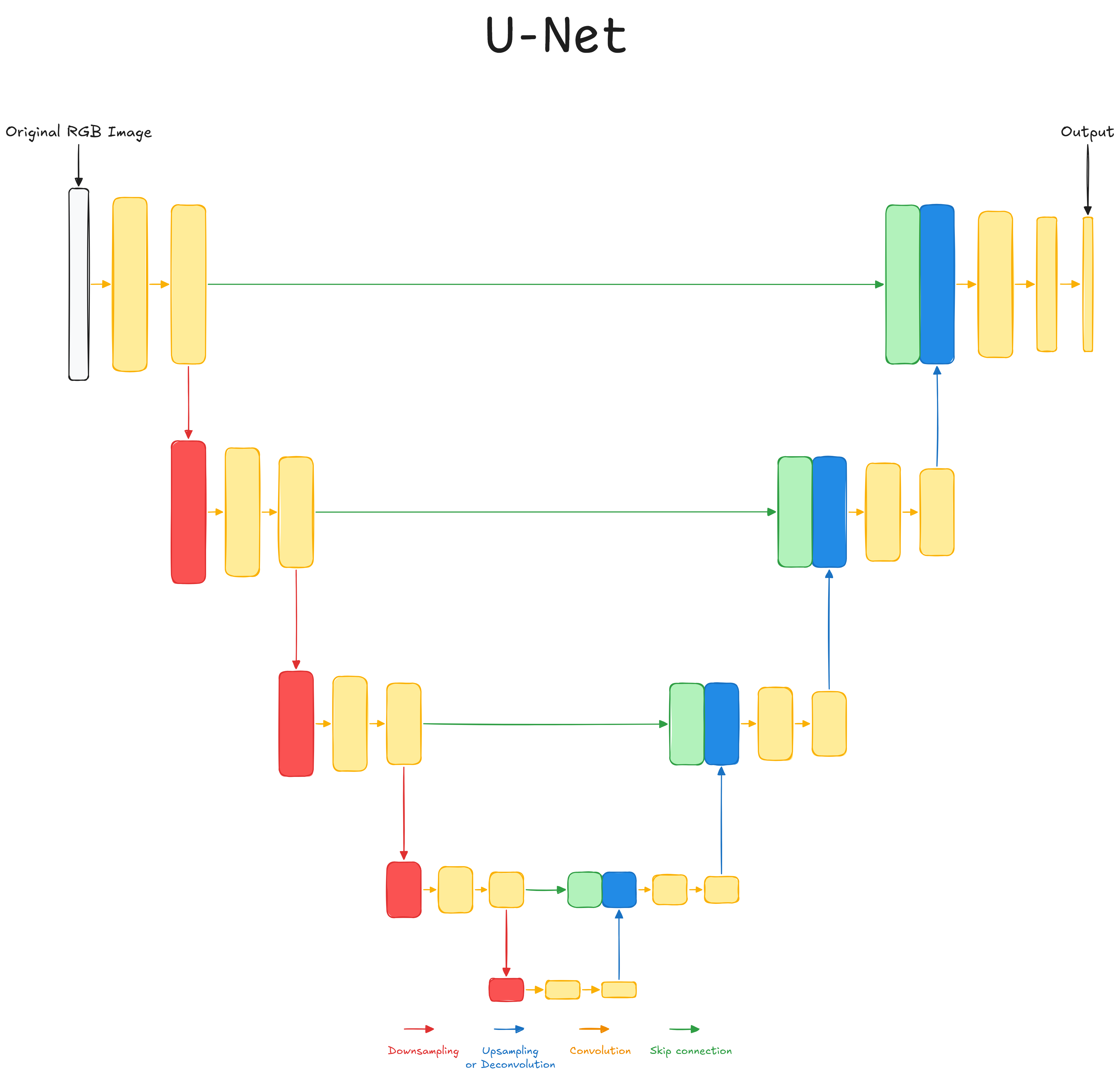
U-Net

It was developed to analyze medical images and segmentation, step in which we add classification to pixels. To train these segmentation models we use target maps that have the desired classification maps.

Tip

During a skip-connection, if the dimension resulting from the upsampling is smaller, it is possible to crop and then concatenate.

Architecture

• Encoder:
  We have several convolutional and pooling layers to make the representation smaller. Once small enough, we'll have a FCNN
• Decoder:
  In this phase we restore the representation to the original dimension (up-sampling). Here we have many deconvolution layers, however these are learnt functions
• Skip Connection:
  These are connections used to tell deconvolutional layers where the feature came from. Basically we concatenate a previous convolutional block with the convoluted one and we make a convolution of these layers.

Pseudo Algorithm

IMAGE = [[...]]

skip_stack = []
result = IMAGE[:]

# Encode 4 times
for _ in range(4):

    # Convolve 2 times
    for _ in range(2):
        result = conv(result)

    # Downsample
    skip_stack.append(result[:])
    result = max_pool(result)

# Middle convolution
for _ in range(2):
    result = conv(result)

# Decode 4 times
for _ in range(4):

    # Upsample
    result = upsample(result)

    # Skip Connection
    skip_connection = skip_stack.pop()
    result = concat(skip_connection, result)

    # Convolve 2 times
    for _ in range(2):
        result = conv(result)

# Last convolution
RESULT = conv(result)

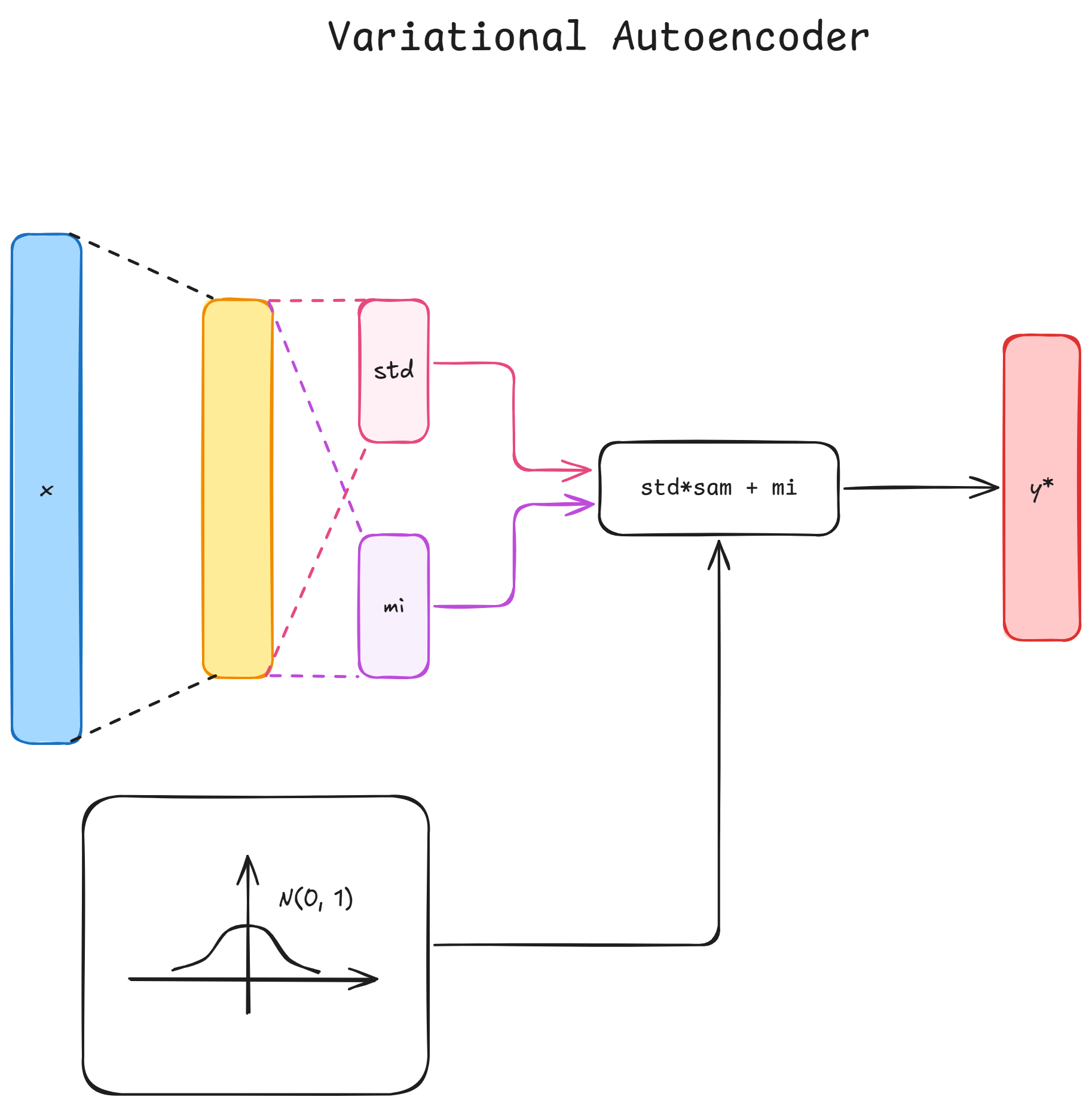
Variational Autoencoders

Until now we were reconstructing points in the latent space to points in the target space.

However, these means that the immediate neighbours of the data point are meaningless.

The idea is to make it such that all immediate neighbour regions of our data point will be decoded as our data point.

To achieve this, our point will become a distribution over the latent-space and then we'll sample from there and decode the point. We then operate as normally by backpropagating the error.

Regularization Term

We use Kullback-Leibler to see the difference in distributions. This has a closed form in terms of mean and covariance matrices

The importance of regularization makes it so that these encoders are both continuous and complete (each point is meaningful). Without it we would have too similar results in our regions. Also this makes it so that we don't have regions too concentrated and similar to a point, nor too far apart from each other

Loss

L(x) = ||x - \hat{x}||^{2}_{2} + KL[N(\mu_{x}, \Sigma_{x}), N(0, 1)]

Tip

The reason behind KL as a regularization term is that we don't want our encoder to cheat by mapping different inputs in a specific region of the latent space.

This regularization makes it so that all points are mapped to a gaussian over the latent space

On a side note, KL is not the only regularization term available, but is the most common.

Probabilistic View

• \mathcal{X}: Set of our data
• \mathcal{Y}: Latent variable set
• p(x|y): Probabilistic encoder, tells us the distribution of x given y
• p(y|x): Probabilistic decoder, tells us the distribution of y given x

Note

Bayesian a Posteriori Probability

  \underbrace{p(A|B)}_{\text{Posterior}} = \frac{
      \overbrace{p(B|A)}^{\text{Likelihood}}
      \overbrace{\cdot p(A)}^{\text{Prior}}
  }{
      \underbrace{p(B)}_{\text{Marginalization}}
  }
  = \frac{p(B|A) \cdot p(A)}{\int{p(B|u)p(u)du}}

• Posterior: Probability of A being true given B
• Likelihood: Probability of B being true given A
• Prior: Probability of A being true (knowledge)
• Marginalization: Probability of B being true

By making the assumption of the probability of y of being a gaussian with 0 mean and identity deviation, and assuming x and y independent and identically distributed:

• p(y) = \mathcal{N}(0, I) \rightarrow p(x|y) = \mathcal{N}(f(y), cI)

Since we need an integral over the denominator, we use approximate techniques such as Variational Inference, easier to compute.

Variational Inference

This approach tries to approximate the goal distribution with one that is very close.

Let's find p(z|x), probability of having that latent vector given the input, by using a gaussian distribution q_x(z), defined by 2 functions dependent from $x$

q_x(z) = \mathcal{N}(g(x), h(x))

These functions, g(x) and h(x) are part of these function families g(x) \in G and h(x) \in H. Now our final target is then to find the optimal g and h over these sets, and this is why we add the KL divergence over the loss:

L(x) = ||x - \hat{x}||^{2}_{2} + KL\left[N(q_x(z), \mathcal{N}(0, 1)\right]

Reparametrization Trick

Since y (\hat{x}) is technically sampled, this makes it impossible to backpropagate the mean and std-dev, thus we add another variable, sampled from a standard gaussian \zeta, so that we have

y = \sigma_x \cdot \zeta + \mu_x

For \zeta we don't need any backpropagation, thus we can easily backpropagate for both mean and std-dev