Control-Network-Systems/docs/Chapters/1-MODERN-CONTROL.md

Modern Control

Normally speaking, we know much about classical control, in the form of:

\dot{x}(t) = ax(t) + bu(t) \longleftrightarrow sX(s) - x(0) = aX(S) + bU(s)

With the left part being a derivative equation in continuous time, while the right being its tranformation in the complex domain field.

Note

\dot{x}(t) = ax(t) + bu(t) \longleftrightarrow x(k+1) = ax(k) + bu(k)

These are equivalent, but the latter one is in discrete time.

A brief recap over Classical Control

Be Y(s) our output variable in classical control and U(s) our input variable. The associated transfer function G(s) is:

G(s) = \frac{Y(s)}{U(s)}

Root Locus

Bode Diagram

Nyquist Diagram

State Space Representation

State Matrices

A state space representation has 4 Matrices: A, B, C, D with coefficients in \R:

• A: State Matrix [x_rows, x_columns]
• B: Input Matrix [x_rows, u_columns]
• C: Output Matrix [y_rows, x_columns]
• D: Direct Coupling Matrix [y_rows, u_columns]

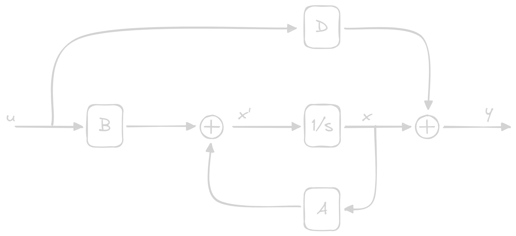
\begin{cases}
\dot{x}(t) = Ax(t) + Bu(t) \;\;\;\; \text{Dynamic of the system}\\
      y(t) = C{x}(t) + Du(t) \;\;\;\; \text{Static of the outputs}
\end{cases}

This can be represented with the following diagrams:

Continuous Time:

---

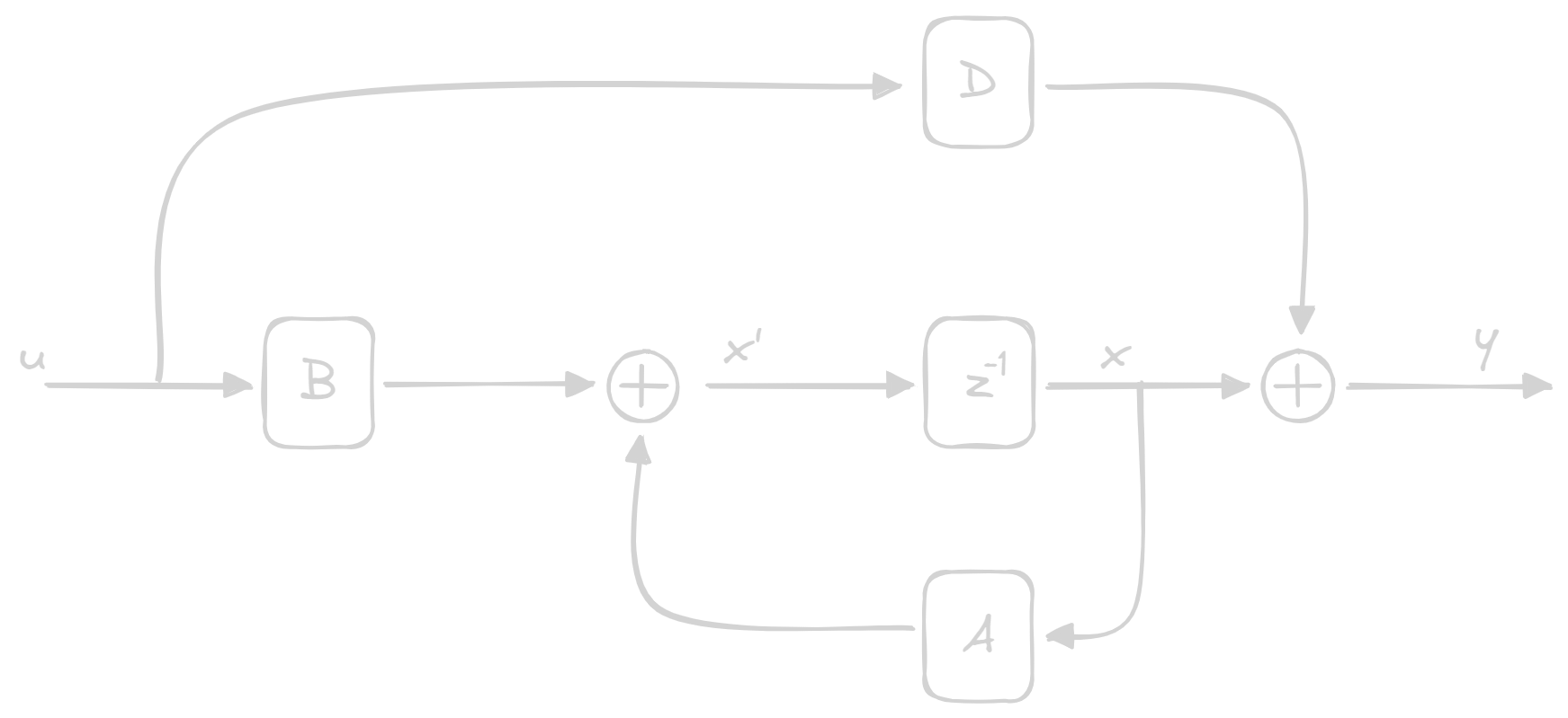
Discrete time:

State Vector

This is a state vector [x_rows, 1]:

x(t) =  \begin{bmatrix}
            x_1(t)\\
            \dots\\
            x_x(t)
        \end{bmatrix}

\text{or} \:

x(k) =  \begin{bmatrix}
            x_1(k)\\
            \dots\\
            x_x(k)
        \end{bmatrix}

Basically, from this we can know each next step of the state vector, represented as:

x(k + 1) = f\left( 
    x(k), u(k)
\right) = Ax(k) + Bu(k)

Examples

Cart attached to a spring and a damper, pulled by a force

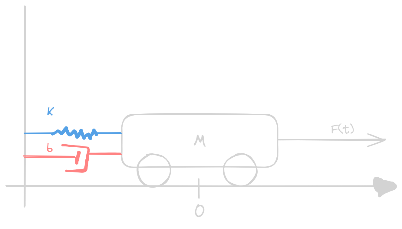
Formulas

• Spring: $\vec{F} = -k\vec{x}$
• Fluid Damper: $\vec{F_D} = -b \vec{\dot{x}}$
• Initial Force: \vec{F_p}(t) = \vec{F_p}(t)
• Total Force: m \vec{\ddot{x}}(t) = \vec{F_p}(t) -b \vec{\dot{x}} -k\vec{x}

Tip

A rule of thumb is to have as many variables in our state as the max number of derivatives we encounter. In this case 2

Solve the equation for the highest derivative order

Then, put all variables equal to the previous one derivated:

x(t) =  \begin{bmatrix}
            x_1(t)\\
            x_2(t) = \dot{x_1}(t)\\
            \dots\\
            x_n(t) = \dot{x}_{n-1}(t)
        \end{bmatrix}
\;
\dot{x}(t) =  \begin{bmatrix}
            \dot{x_1}(t) = x_2(t)\\
            \dot{x_2}(t) = x_3(t)\\
            \dots\\
            \dot{x}_{n-1}(t) = \dot{x}_{n}(t)\\
            \dot{x}_{n}(t) = \text{our formula}
        \end{bmatrix}

Now in our state we may express position and speed, while in our next_state we'll have speed and acceleration:

x(t) =  \begin{bmatrix}
            x_1(t)\\
            x_2(t) = \dot{x_1}(t)
        \end{bmatrix}
\;
\dot{x}(t) =  \begin{bmatrix}
            \dot{x_1}(t) = x_2(t)\\
            \dot{x_2}(t) = \ddot{x_1}(t)
        \end{bmatrix}

Our new state is then:

\begin{cases}
\dot{x}_1(t) = x_2(t)\\
\dot{x}_2(t) = \frac{1}{m} \left( \vec{F}(t) - b x_2(t) - kx_1(t) \right)
\end{cases}

let's say we only want to check for the position and speed of the system, our State Space will be:

A = \begin{bmatrix}
0 & 1 \\
- \frac{k}{m} & - \frac{b}{m} \\
\end{bmatrix}

B = \begin{bmatrix}
0 \\
\frac{1}{m} \\
\end{bmatrix}

C = \begin{bmatrix}
1 & 0 \\
0 & 1
\end{bmatrix}

D = \begin{bmatrix}
0
\end{bmatrix}

let's say we only want to check for the position of the system, our State Space will be:

A = \begin{bmatrix}
0 & 1 \\
- \frac{k}{m} & - \frac{b}{m} \\
\end{bmatrix}

B = \begin{bmatrix}
0 \\
\frac{1}{m} \\
\end{bmatrix}

C = \begin{bmatrix}
1 & 0 
\end{bmatrix}

D = \begin{bmatrix}
0
\end{bmatrix}

Tip

In order to being able to plot the \vec{x} against the time, you need to multiply \vec{\dot{x}} for the time_step and then add it to the state¹

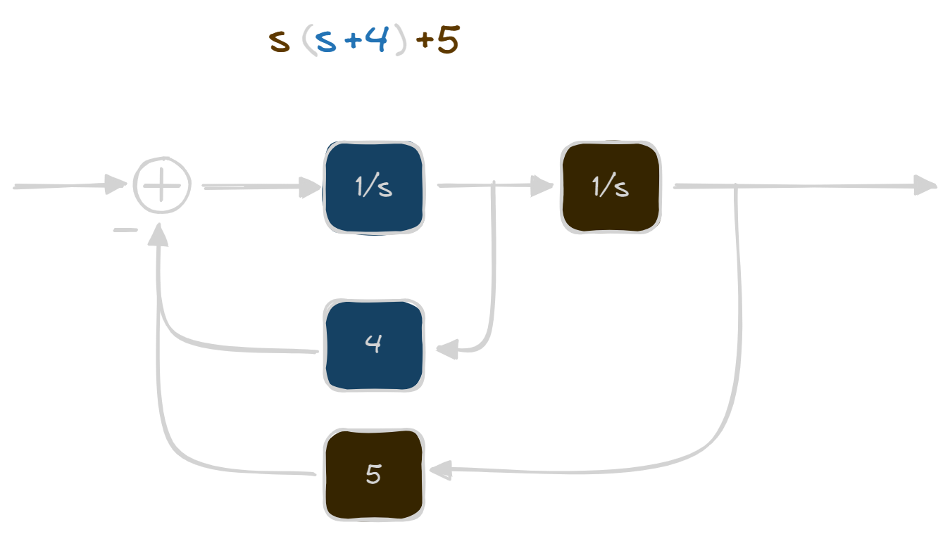
Horner Factorization

let's say you have a complete polynomial of order n, you can factorize in this way:

\begin{align*}
p(s) &= s^5 + 4s^4 + 5s^3 + 2s^2 + 10s + 1 =\\

&= s ( s^4 + 4s^3 + 5s^2 + 2s + 10) + 1 = \\

&= s ( s (s^3 + 4s^2 + 5s + 2) + 10) + 1 = \\

&= s ( s (s (s^2 + 4s + 5) + 2) + 10) + 1 = \\

&= s ( s (s ( s (s + 4) + 5) + 2) + 10) + 1

\end{align*}

If you were to take each s with the corresponding number in the parenthesis, you'll make this block:

Case Studies

• PAGERANK
• Congestion Control
• Video Player Control
• Deep Learning

---

1. Stack Exchange | How to plot state space variables against time on unit step input? | 05 January 2025 ↩︎